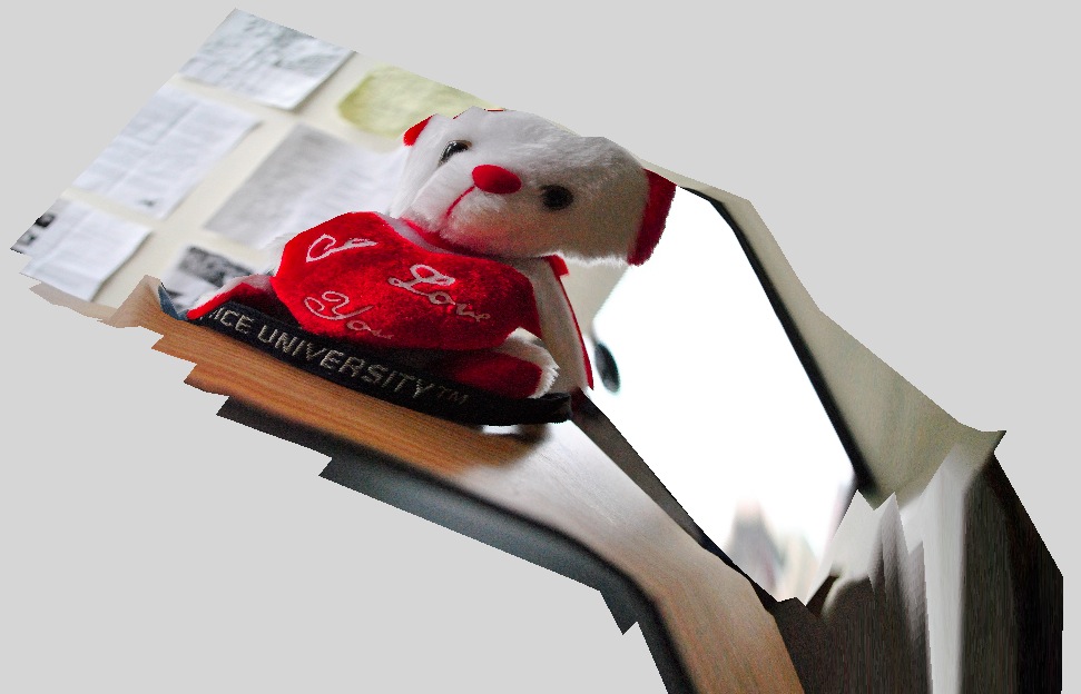
Using the griddata and surf functions in Matlab, we are able to interpolate the z data of each feature in 3D space, to see what the rest of the regions in between features is doing. Then by laying an original picture over this data we can see visually how deep regions of our photographs are in space.
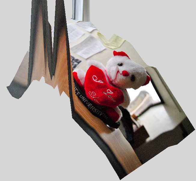
Aside from the extremes in the very front and back left corner, depths make sense. Shallow over bear, deeper to the left with the near by wall, and very deep to the right with the door.
As was mentioned earlier, the least squares method is more unstable and is visably so with the extremes in the front of the photo and in the back left corner. However the rest of the photo makes intuitive sense. All the reported Z values are off by a scale factor due to the explained ambiguity.
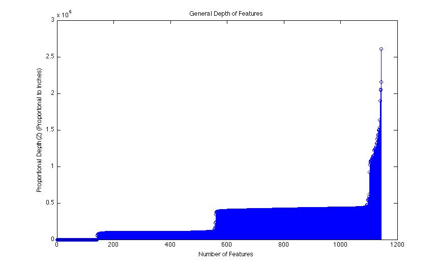
Region 200 to 600 is the bear’s depth, 600 to 1000 is the background(wall), and 1000 to the end is the extreme depth represented by the hallway.
Porportionally this graph makes sense because the wall was in fact about 3 times as far as the bear was to the camera, and the depth of the hallway was obviously extreme compared to the wall because we could not see the end of it in the photo, it seemed to go to infinity.
Therefore these results and the corresponding depth map of the two steoro images fits our expectations.
This method is much more stable and demesntrates better quick changes in depth than the previous method. This algorithm understand that there is a huge drop from the depth of the bear to the hallway to the right of it.
Data for this section is not important because all values do not take into consideration 3D space, simply the disparities of the features and the camera positions.
To further test our alogorithm on a large depth, we shot two stero images of the Duncan wall way and used the Disparity method as shown above to get an idea of the relative depths.
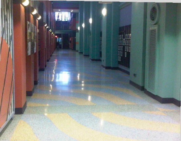
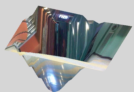
Notice large Depth that terminates correctly where the end of the hall should be.
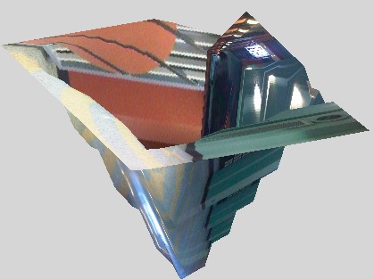
Notice how Side Wall Depth is accurate with jagged depths that match the surface of the real walls in Duncan Hall.
Once again we see that this algorithm is very powerful in transforming two stero images into a depth map, that is also very accurate in its proportional depth from camera.