5.1 Introduction and Preparation of SAR Data
In order to simulate the processing of SAR data, we received SAR data from the ECE department at Ohio State University. The data they gave us was acquired through a computer simulated y-by past a CAD model of a backhoe.

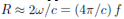
Figure 5.1
The data we received from OSU was in digital format, meaning the analog mixing and low pass filtering was already completed and we received digitized versions of Cθ(t). This function was shown to be equivalent to Pθ(U), the Fourier transform of our projection slices pθ(u). The matlab le that contained this information was a 512x1541 matrix iq_lin, a vector of various Pθ signals for different values of θ, the viewing angle. There were 1541 different viewing angles, listed in az_lin, that stepped by 1/14 for each element and varied from -10 to 100, a median viewing angle of 45. We also received a vector of length 512 called f that contained the microwave frequencies (7-13 GHz) that were transmitted and received. By using the wideband approximation, we made the transformation from time frequency to spatial frequency via
where R is the radial spatial frequency and f is the microwave frequency content. By the projection slice theorem, we have that the various Pθ are arranged radially in a polar grid along the various angles θ. We then get that our data lies on a domain
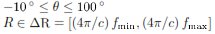
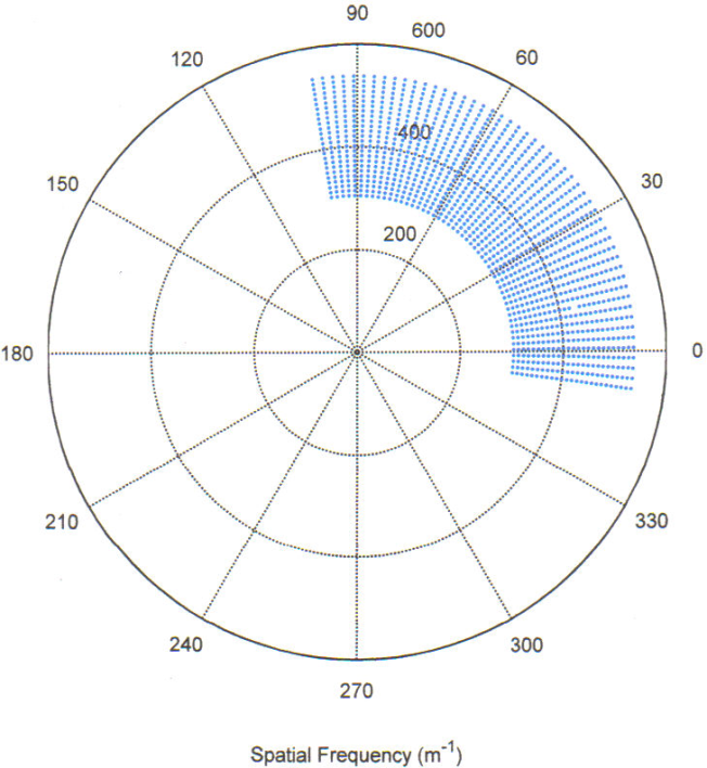
Figure 5.2
5.2 Processing of SAR Data
Knowing that our data is the Fourier transform of our image, after the proper preparation we want to take the inverse Fourier transform. To do this simply and efficiently (we don't want Matlab running for hours!) we linearly interpolate the data to a Cartesian grid. This is done in our Matlab function sar_lin (code found in appendix). The idea is to find an inscribed rectangular grid inside our polar data. We chose to use the square centered at 45 inscribed in our ribbon. To interpolate we made a Cartesian grid at this location and computed the polar representation of each point in order to find its 4 nearest polar neighbors. Once those neighbors were found, the Cartesian point's value was determined by linearly interpolating in the R-direction for the two θ values and then linearly interpolating in the θ-direction. The end result of our program's running of this is shown below.
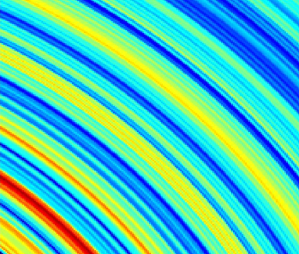
Figure 5.3
After linearly interpolating each point in the Cartesian grid we have formed, we now have our data in a form that allows us to take the 2-d inverse DFT by the fast Fourier transform method. This is what saved us computation time (program ran in about 15 seconds) and is the reason we interpolated to Cartesian coordinates to begin with. Below is the image after taking the inverse Fourier transform.
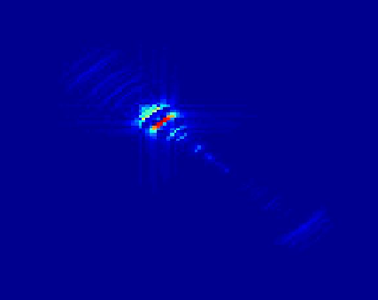
Figure 5.4