Chapter - 6
THEORY OF GENERAL EQUILIBRIUM
(Debreau & W. Leontief)
Debreau
Debreau, won the Nobel Prize earlier than his inspirer Allais. Debreau has made a significant contribution to General Equilibrium theory, which is discussed in his short and highly mathematical book, Theory of Value. The seeds of General Equilibrium theory can be traced to Adam Smith’s formulation of the laws of Markets, where “The private interests and passions of men are led by an invisible hand in the direction which is most agreeable to the interest of the whole society”.
Smith’s idea that everything depends on all other things was not followed in United Kingdom. In Marshall’s time, markets were analyzed mostly on-at-a-time – a partial equilibrium analysis. The inter connections among markets were not explored.
The theory of General Equilibrium is developed thoroughly in 1874 by the French mathematician and economist, Leon Walras and Villfred Pareto. They have explained how millions of individual market decisions can achieve overall equilibrium of the system. Debreau’s research in General Equilibrium Theory (Done jointly with Arrow) throws light on a set of conditions required under which Perfect Market could exist. The Arrow -Debreau results show that, given some pre-conditions, the results of market mechanism is Paretooptimal.
From the works of Arrow – Debreau on General Equilibrium, we learn that a particular economic change will have remote repercussions that may be a more significant than the initial change. After their work the market mechanism became the panacea for all the ills of the economies. In fact, their assumptions were very restrictive. If perfect markets were not there markets would be inefficient.
The proof of existence of general equilibrium in a competitive model by Arrow – Debreau is highly mathematical, requiring knowledge of set theory.
Wassily Leontief
Wassily Leontief’s work, Input-Output Analysis is a major effort towards empirical quantification of General equilibrium theory. It studies general equilibrium phenomena in the empirical analysis of production. Input output model seeks to take account of the interdependent nature of the production plans and activities of many industries which constitute an economy. The interdependence arises out of the fact that each industry employs the outputs of other industries as its inputs and supplies its outputs to other industries as raw material for their products. The residual output is available for final consumption.
Input-output analysis is a useful tool and served as base for planning in many countries.
Input-Output analysis is explained-below using an example. (General readers may skip the illustration below). Suppose, there are two sectors Agriculture (A) and manufacturing (M) and they use Primary inputs like Labor. Also there is Final Consumption of goods given exogenously. (C) Details of Input-Output Table are given below.
Table 1, Input-Output Table
|
Input
|
Output
|
|
Sector
|
A
|
M
|
C
|
X
|
|
Agriculture (A)
|
200
|
100
|
150
|
450
|
|
Manufactures (M)
|
180
|
120
|
100
|
400
|
|
Value added (Primary input)
|
70
|
180
|
-
|
-
|
|
Gross Income
|
450
|
400
|
-
|
850
|
In the above Table Rows represent output flows of each Sector and Columns show the input use of each Sector. The gross National Income (Output) is Rs.850 crores.
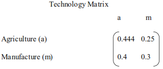
Leontief assumed that all Factor proportions are technologically fixed. Ratio of each input divided by output gives the Technical Coefficient. for eg. In the first column (and first Row) 200/450 gives a Technical Co-efficient of 0.444, and so on for others.
The Technology Co-efficient Matrix is presented below. (Matrix A)

Suppose, a Planner or Policy maker wants that consumption of Agricultural goods should be increased to Rs.200 and Manufactured goods to Rs.150. using the Technical Co-efficient and the change consumption requirements, we write the equations and solve for outputs.
0.444Xa + 0.25Xm + Ca - Xa = 0
0.4Xa + 0.3Xm +Cm –Xm = 0
We can solve the above simultaneous equations by conventional methods in algebra.
Solving, we get Xa = 618 and Xm = 567
Agricultural sector has to produce output of 618 and Manufacturing sector has to produce output of 567 in order to meet the changed consumption.
Those familiar with Matrix methods, they may use the following procedure to solve the equations.
- Deduct technology Matrix from Identity matrix. We get Leontief Matrix.
- Calculate the Inverse for Leontif Matrix
- We can find the output vector by post multiplying the Inverse of Leontief Matrix by consumption Vector.
Of late, the general equilibrium method is used in macro-economic dynamics. Such models are known as Dynamic Stochastic General Equilibrium Models (D.S.G.E. models). In their construction advanced mathematical methods are used, such as stochastic difference and differential equations.


