Chapter 5
Q3: What can We Expect from
Modelling Climate Change 1
5.1 Modeling climate to determine the degree and effect of future climate change: What can we expect?
5.1.1 Short answer
The future global surface temperature and some other climate variables can be modeled with reasonable confidence for various scenarios for the future energy policy of the globe. These results are only as good as our ability to predict the actual energy consumption patterns of the whole world.
5.1.2 Detailed answer
Predicting the future with any real precision is virtually impossible. Future climate change depends on several human activities, the most important of which are the use of fossil fuels for energy and continued land use change in the form of new urban communities or reductions of forest areas. The current best way to approach a prediction of future climate is to develop a series of plausible scenarios of future human activity and then run simulations using a multi-model approach to obtain average climate outcomes for each. The results will be an array of different climate futures that can provide a basis for choosing how much climate change we wish to tolerate and what mitigation and life style changes will be necessary to achieve that end.
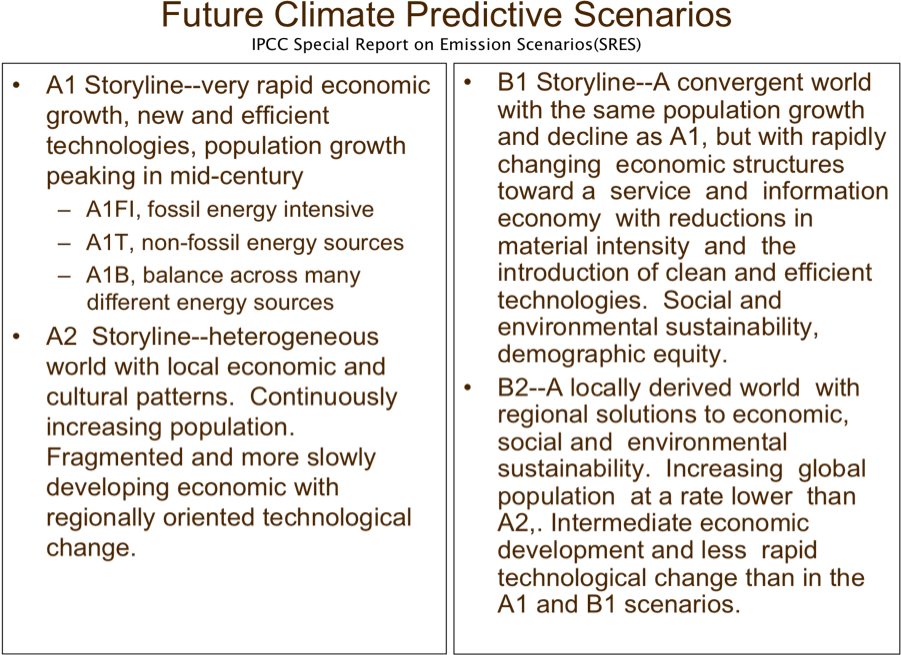
Figure 5.1: IPCC adopted scenarios of the Earth's energy future for the purpose of predicting the resultant climates
______________________________________
Several scenarios have been proposed for the global future. The IPCC “Special Report on Emissions Scenarios”. (2000) presents six scenarios for the future. These are named A1B, A1F1, A1T, A2, B1 and B2 and are briefly described in Figure 5.1. The carbon emission predictions derived from these scenarios are compared over the next century in Figure 5.2. The carbon dioxide (CO2) emission values are in GtC (Gigatons carbon) per year. A gigaton of carbon refers to only the weight of carbon in the carbon dioxide emissions. The amount of carbon dioxide can be obtained by multiplying the amount of carbon by the ratio of the molecular weights of carbon dioxide to carbon (44/12 = 3.67). Thus the value of the current emission (7 GtC) is really 25.7 Gt carbon dioxide.
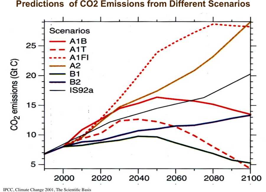
Figure 5.2: The development of carbon emission scenarios over the next century.
_____________________________
The corresponding changes in the concentration of atmospheric carbon dioxide are depicted in Figure 5.3.
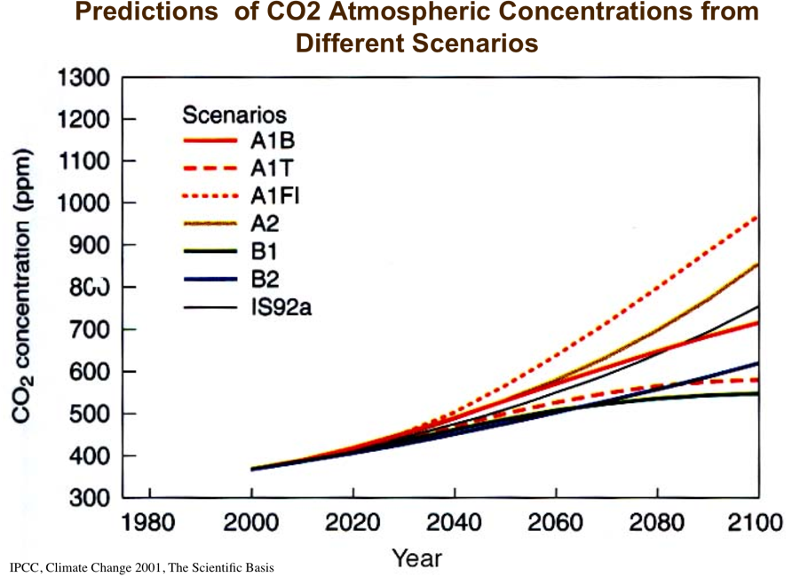
Figure 5.3: Values over the next century of predicted atmospheric concentrations of carbon dioxide.
_____________________________
The most optimistic emission curtailments are found in both A1T and B2. A1T indicates early increases in carbon emissions followed by a steady decline as population peaks and declines and as fossil fuel is replaced by renewable energy sources. B2 stresses moderation on all fronts – social, economic and environmental. The most distressing scenarios for carbon emissions are A1F1, which maintains intensive fossil energy, and A2, which is probably the closest scenario to -business as usual.. The last two scenarios, A1B and B1, end up the century with intermediate carbon emissions. Because A1B peaks and is decreasing as 2100 approaches, it has greater promise of even lower values in the following century. Yet, B1 is a very probably the most realistic approximation of the best that can be expected for the world. Each of these scenarios has been subject to multiple computer simulations and the best estimated average global surface temperature increase (oC) as well as the statistical error bar (to the right) and the envelope of uncertainty for each model are exhibited in Figure 5.4.
______________________________
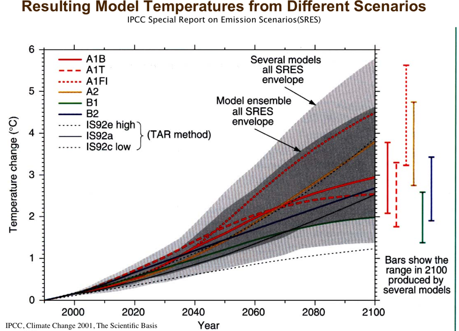
Figure 5.4: Modeled global temperature values for the standard IPCC fossil fuel scenarios.
______________________________
Although none of these scenarios is thought to accurately depict the actual future of the world, they do give a reasonable range of behavior options we may adapt in order to mitigate the possible climate change. The model process also provides us with good estimates of the relationship between actual atmospheric carbon dioxide concentrations and resulting expected temperature change. Models also can provide us with information about changes in other climate factors such as regional changes in precipitation and evapotranspiration, soil moisture, sea surface temperature and acidity, and others, all leading to changes in agricultural productivity, sea level and coastal flooding, public health, species viability and ecosystem health. The top of Figure 5.5 presents the maximum, minimum and most probable average surface global temperature associated with various atmospheric carbon dioxide levels. The bottom part of Figure 5.5 then relates these temperature changes to various observable impacts in the form of arrows starting out yellow at temperatures associated with small effects to red at temperatures at which the effects become severe. For example, the first food effect starts with minor falling crop yields in some regions at about 1.5 oC temperature change to severe crop failures at temperature changes over 5 oC. Scenarios A1T or B2 are the most optimistic scenarios considered. They both show a modest increase in carbon dioxide emission peaking around 2040 and coming back to current levels by 2100 (Figure 5.2). Even under these -best cases., the atmospheric concentration by 2100 will have reached a value of approximately 550 parts per million (Figure 5.3) and the temperature change due to the addition of these gases will have reached about 2.5 oC (4.5 oF) with an uncertainty of  0.8 oC (Figure 5.3). The worse case scenario considered is represented by A1F1. This scenario is essentially “business as usual” or no significant changes from current energy practices. In this scenario, carbon dioxide emission reaches over 28 billion tons of carbon (102 tons of carbon dioxide equivalents) per year (Figure 5.2) with an atmospheric carbon dioxide concentration over 900 parts per million (Figure 5.3). The model temperature rise predicted for the year 2100 by this scenario is 4.5 oC (8.1 oF) (Figure 5.4). This scenario is where we are currently headed and is completely unacceptable. Figure 5.5 shows what kind of a world we can expect. The Amazon rainforest is gone, hurricanes have increased in intensity, crop yields are down, sea level threatens coastal cities, and there is a possibility of passing the tipping point to a large-scale abrupt climate change.
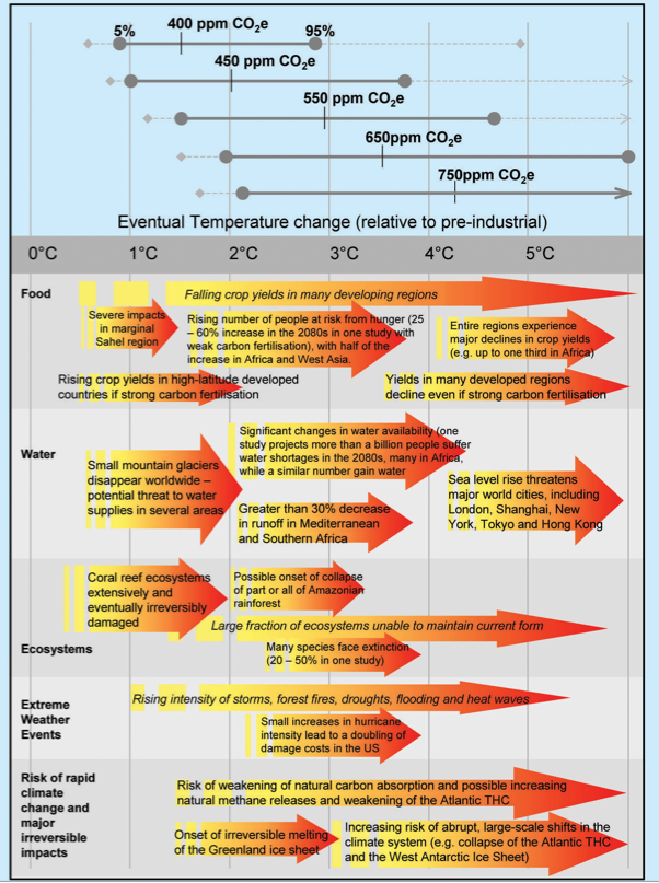
Figure 5.5: Examples of impacts associated with various projected global atmospheric carbon dioxide concentrations and resulting temperature change (Stern. Sir N. (2006) Stern Review: The Economics of Climate Change). Available for free at Connexions