T he behavior of a buyer is influenced by many factors: the price of the
good, the prices of related goods (compliments and substitutes), incomes of
the buyer, the tastes and preferences of the buyer, the period of time and a
variety of other possible variables. The quantity that a buyer is willing and able
to purchase is a function of these variables.
An individual’s demand function for a good (Good X) might be written:
QX = fX(PX, Prelated goods, income (M), preferences, . . . )
•
QX = the quantity of good X
•
PX = the price of good X
•
Prelated goods = the prices of compliments or substitutes
•
Income (M) = the income of the buyers
•
Preferences = the preferences or tastes of the buyers
The demand function is a model
that “explains” the change in the
riceP
$8
dependent variable (quantity of the
$7
good X purchased by the buyer)
$6
$5
“caused” by a change in each of the
$4
independent variables. Since all the
$3
$2
independent variable may change at
Demand
$1
the same time it is useful to isolate
2
4
6 8 10 12 14 16 18
Quantity/ut
Figure III.A.1
the effects of a change in each of the
150
8.1.1 Individual Demand Function
independent variables. To represent the demand relationship graphically, the
effects of a change in PX on the QX are shown. The other variables, (Prelated goods,
M, preferences, . . . ) are held constant. Figure III.A.1 shows the graphical
representation of demand. Since (Prelated goods, M, preferences, . . . ) are held
constant, the demand function in the graph shows a relationship between PX
and QX in a given unit of time (ut).
The demand function can be viewed from two perspectives.
The demand is usually defined as a schedule of quantities that buyers are
willing and able to purchase at a schedule of prices in a given time
interval (ut), ceteris paribus.
QX = f(PX), given incomes, price of related goods, preferences, etc.
Demand can also be perceived as the maximum prices buyers are willing
and able to pay for each unit of output, ceteris paribus.
PX = f(QX), given incomes, price of related goods, preferences, etc.
It is important to remember that the demand function is usually thought of
as Q = f(P) but the graph is drawn with quantity on the X-axis and price on
the Y-axis. While demand is frequently stated Q = f(P), remember that
the graph and calculation of total revenue (TR) and marginal revenue (MR) are
calculated on the basis of a change in quantity (Q). TR = f(Q) The calculation
of “elasticity” is based on a change in quantity (Q) caused by a change in the
price (P). It is important to clarify which variable is independent and which is
dependent in a particular concept.
8.1.2 MARKET DEMAND FUNCTION
W hen property rights are nonattenuated (exclusive, enforceable and
transferable) the individual’s demand functions can be summed horizontally to
obtain the market demand function.
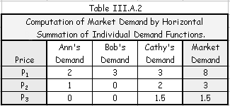
In Figure III.A.2 and Table III.A.2, a market demand function is
constructed from the behavior of three people (the participants in a very small
151
8.1.2 Market Demand Function
market. At a price of P1, Ann will voluntarily buy 2 units of the good based on
her preferences, income and the prices of related goods. Bob and Cathy buys
3 units each. Their demand functions are represented by DA, DB and DC in
Figure III.A.2.
rice
Figure III.A.2
P
DB
P3 D d
A
d
P2
Market Demand
DM
P1
DC
d
1
2
3
8
Q/ut
The total amount demanded by the three individuals at P1 is 8 units
(2+3+3). At a higher price each buys a smaller quantity. The demand
functions can be summed horizontally if the property rights to the good are
exclusive: Ann’s consumption of a unit precludes Bob or Cathy from the
consumption of that good. In the case of public (or collective) goods, the
consumption of national defense by one person (they are protected) does not
preclude others from the same good.
The behavior of a buyer was represented by the function:
QX = fX(PX, Prelated goods, income (M), preferences, . . . ). For the market
the demand function can be represented by adding the number of buyers (#B,
or population),
QX = fX(PX, Prelated goods, income (M), preferences, . . . #B)
152
8.1.2 Market Demand Function
Where #B represents the number of buyers. Using ceteris paribus the
market demand may be stated
QX = f(PX), given incomes, price of related goods, preferences, #B etc.
8.1.3 CHANGE IN QUANTITY DEMAND
W hen demand is stated Q = f(P) ceteris paribus, a change in the price of
the good causes a “change in quantity demanded.” The buyers respond to
a higher (lower) price by purchasing a smaller (larger) quantity. Demand is an
inverse relationship between price and quantity demanded. Only in unusual
circumstances (a highly inferior good, a Giffen good) may a demand function
have a positive relationship.
A change in quantity demanded is a movement along a demand function
caused by a change in price while other variables (incomes, prices of related
goods, preferences, number of buyers, etc) are held constant. A change in
quantity demanded is shown in Figure III.A.3.
An increase in quantity demanded is a movement
rice P
along a demand curve (from point A to B) caused
$8
by a decrease in the price from $7 to $4.
$7
A decrease in quantity demanded is a movement
A
$6
along the demand function (from point B to A)
caused by an increase in price from $4 to $7.
$5
$4
B
$3
$2
Demand
$1
2
4
6 8 10 12 14 16 18
Quantity/ut
Figure III.A.3
153
8.1.4 Change in Demand
8.1.4 CHANGE IN DEMAND
A change in demand is a “shift” or movement of the demand function. A
shift of the demand function can be caused by a change in:
• incomes
• the prices of related goods
• preferences
• the number of buyers.
• Etc . . .
A“change in demand” is shown in Figure III.A.4. Given the original demand
(Demand), 10 units will be purchased at a price of $5. An increase in demand
(DINCREASE) is to the right and at every price a larger quantity will be purchased.
At $5, eighteen units are purchased. A decrease in demand is a shift to the
left. At a price of $5 only 4 units are purchased. A smaller quantity will be
bought at each price.
Given a demand function (Demand), an increase in demand is
rice
shown as D
P
INCREASE. At each price a larger quantity is
purchased.
$8
Increase
A decrease in demand is shown as DDECREASE. At each
$7
Decrease
possible price the quantity purchased is less.
$6
H
$5
G
J
$4
$3
DINREASE
$2
Demand
$1
DDECREAS
E
2
4
6
8 10 12 14 16 18
Quantity/ut
Figure III.A.4
154
8.1.5 Inferior, Normal and Superior Goods
8.1.5 INFERIOR, NORMAL AND SUPERIOR GOODS
A change in income will usually shift the demand function. When a good
is a “normal” good, there is a positive relationship between the change in
income and change in demand: an increase in income will increase (shift the
demand to the right) demand. A decrease in income will decrease (shift the
demand to the left) demand.
An inferior good is characterized by an inverse or negative relationship
between the change in income and change in demand. An increase in the
income will decrease demand while a decrease in income will increase
demand.
rice P
$8
Increase
$7
Decrease
$6
H
$5
G
J
$4
$3
DINCREAS
$2
Demand E
$1
DDECREAS
E
2
4
6
8 10 12 14 16 18
Quantity/ut
Figure III.A.2
A superior good is a special case of the normal good. There is a positive
relationship between a change in income and the change in demand but, the
percentage change in the demand is greater than the percentage change in
income. In Figure III.A.2 an increase in income will shift the Demand function
(“Demand”) for a normal good to the right to DINCREASE. For an inferior good, a
decrease in income will shift the demand to the right. For a normal good a
decrease in income will shift the demand to DDECREASE.
155
8.1.6 Compliments and Substitutes
8.1.6 COMPLIMENTS AND SUBSTITUTES
T he demand for Xebecs (QX) is determined by the PX, income and the
prices of related goods (PR). Goods may be related as substitutes (consumers
perceive the goods as substitutes) or compliments (consumers use the goods
together). If goods are substitutes, (shown in Figure III.A.3) a change in PY (in
Panel B) will shift the demand for good X (in Panel A).
Substitutes
Price
Price
Goods X and Y are substitutes, An increase in
PY (from PY1 to PY2) decreases the quantity
PY2
demanded for Y from Y
D
1 to Y2. The demand for
Y
good X increases to DX*. At PX the amount
purchased increases from X
P
2 to X3. A decrease
X
D
in PY shifts DX to DX** (Amount of X
X*
P
decreases to X1).
Y1
D
D
X**
X
X1
X2
X3 Q
Y2
Y1
X /ut
QY /ut
Panel A
Panel B
Figure III.A.3
An increase in PY (from PY1 to PY2) will reduce the quantity demanded for
good Y (a move on DY). The reduced amount of Y will be replaced by
purchasing more X. This is a shift of the demand for good X to the right (In
Panel A, this is shown as a shift from DX to DX*, an increase in the demand for
good X). At PX a larger amount (X3) is purchased
A decrease in PY will increase the quantity demanded for good Y. This will
reduce the demand for good X, the demand for good X will shift to the left
(from DX to DX**, a decrease). At PX (and all prices of good X) a smaller
amount of X (X1) is purchased.
In the case of compliments, there is an inverse relationship between the
price of the compliment (PZ in Panel B, Figure III.A.4) and the demand for
156
8.1.6 Compliments and Substitutes
good X. An increase in the price of good Z will reduce the quantity demanded
for good Z. Since less Z is purchased, less X is needed to compliment the
reduced amount of Z (Z2). The demand for X in Panel A decreases for DX to
DX**. An decrease in PZ will increase the quantity demanded of good Z and
result in an increase in the demand for good X (from DX to DX* in Panel A).
Compliments
Price
Price
Goods X and Z are compliments, An increase in
PZ (from PZ1 to PZ2) decreases the quantity
PZ2
demanded for Z from Z
D
1 to Z2. The demand for
Z
good X decreases to DX**. At PX the amount
purchased decreases from X
P
2 to X1. A decrease
X
D
in PZ shifts DX to DX* (Amount of X increases
X*
P
to X3).
Z1
D
DX
X**
X1
X2
X3 Q
Z2
Z1
X /ut
QZ /ut
Panel A
Panel B
Figure III.A.4
8.1.7 EXPECTATIONS
E xpectations about the future prices of goods can cause the demand in
any period to shift. If buyers expect relative prices of a good will rise in future
periods, the demand may increase in the present period. An expectation that
the relative price of a good will fall in a future period may reduce the demand
in the current period.
8.2 SUPPLY FUNCTION
A supply function is a model that represents the behavior of the
producers and/or sellers in a market.
QXS = fS(PX, PINPUTS, technology, number of sellers, laws,
taxes, expectations . . . #S)
PX = price of the good,
157
8.2 Supply Function
PINPUTS = prices of the inputs (factors of production used)
Technology is the method of production (a production
function),
laws and regulations may impose more costly methods of
production
taxes and subsidies alter the costs of production
#S represents the number of sellers in the market.
Like the demand function, supply can be viewed from two perspectives:
Supply is a schedule of quantities that will be produced and offered for sale
at a schedule of prices in a given time period, ceteris paribus.
A supply function can be viewed as the minimum prices sellers are willing
to accept for given quantities of output, ceteris paribus.
8.2.1.1 (1) GRAPH OF SUPPLY
T he relationship between the quantity produced TABLE III.A.5
and offered for sale and the price reflects opportunity
SUPPLY
cost. Generally, it is assumed that there is a positive
FUNCTION
relationship between the price of the good and the PRICE QUANTITY
quantity offered for sale. Figure III.A.5 is a graphical
representation of a supply function. The equation for
$5
0
this supply function is Qsupplied= -10 + 2P. Table III.A5
$10
10
also represents this supply function.
$15
20
8.2.1.2 (2) CHANGE IN QUANTITY SUPPLIED
G
$20
30
iven the supply function, Qxs = fs(Px, Pinputs,
Tech, . . .), a change in the price of the good (PX) will
be reflected as a move along a supply function. In Figures III.A.5 and III.A.6
as the price increases from $10 to $15 the quantity supplied increases from 10
to 20. This can be visualized as a move from point A to point B on the supply
158
8.2 Supply Function
function. A “change in quantity supplied is a movement along a supply
function.” This can also be visualized as a movement from one row to
another in Table III.A.5.
Supply
8.2.1.3 (3) CHANGE IN SUPPLY
Price
C
iven the supply function, Q
$20
xs =
Gf
B
s(Px, Pinputs, Tech, . . ., #S), a
$15
change in the prices of inputs (Pinputs) or $10
A
technology will shift the supply function. A
$5
shift of the supply function to the right will
be called an increase in supply. This means
10
20
30 Q/ut
that at each possible price, a greater
Figure III.A.5
quantity will be offered for sale. In an
equation form, an increase in supply can be shown by an increase in the
quantity intercept. A decrease in supply is a shift to the left: at each possible
price a smaller quantity is offered for sale. In an equation this is shown as a
decrease in the intercept.
Supply
A change in quantity supplied is a movement along
Price
a supply function that is “caused” by a change in the
C
$20
price of the good. In the graph to the right, as price
increases from $10 to $15 the quantity supplied
B
$15
increases from 10 to 20. This can be visualized as a
move from point A to point B along the supply
A
function. A decrease in supply would be a move
$10
from point B to point A as price fell from $15 to $10
$5
10
20
30 Q/ut
Figure III.A.6
159
8.2 Supply Function
A change in supply is a “shift” of the supply
function. A decrease in supply is shown as a
Supply
shift from Supply to S
S
decrease in the graph. At
Price
decrease
C
a price of $15 a smaller amount is offered for
$20
sale. This decrease in supply might be
R
B
H
“caused” by an increase in input prices, taxes,
$15
E
Sincrease
regulations or, . . .
A
An increase in supply can be visualized as a
$10
movement of the supply function from
$5
Supply to Sincrease.
10
20
30 Q/ut
Figure III.A.7
8.3 EQUILIBRIUM
Webster’s Encylopedic Unabridged Dictionary of the English Language
defines equilibrium as “a state of rest or balance due to the equal action of
opposing forces,” and “ equal balance between any powers, influences, etc. ”
T
he New P
algrave : A Dictionary or Economics identifies 3 concepts of
equilibrium:
•
Equilibrium as a “balance of forces”
•
Equilibrium as “a point from which there is no endogenous ‘tendency to change’”
•
Equilibrium as an “ outcome which any given economic process might be said to be
‘tending towards’, as in the idea that competitive processes tend to produce
determinant outcomes.””
In Neoclassical microeconomics, “equilibrium” is perceived as the condition
where the quantity demanded is equal to the quantity supplied: the behavior
of all potential buyers is coordinated with the behavior of all potential sellers.
There is an equilibrium price that equates or balances the amount that agents
want to buy with the amount that is produced and offered for sale (at that
price). There are no forces (from buyers or sellers) that will alter the
160
8.3 Equilibrium
equilibrium price or equilibrium quantity. Graphically, economists represent a
market equilibrium as the intersection of the demand and supply functions.
This is shown in Figure III.A.8.
In the graph to the left, equilibrium is at the
Supply
intersection of the demand and supply
Price
C
functions. This occurs at point B. The
$20
equilibrium price is $15 and the equilibrium
quantity is 20 units.
B