CHAPTER
FOUR
GOAL
In this tutorial we’re looking at a number of techniques to make CPU-bound tasks in Python run much faster. Speed- ups of 10-500* are to be expected if you have a problem that fits into these solutions.
In the results further below I show that the Mandelbrot problem can be made to run 75* faster with relatively little work on the CPU and up to 500* faster using a GPU (admittedly with some C integration!).
Techniques covered:
-
Python profiling (cProfile, RunSnake, line_profiler) - find bottlenecks
-
PyPy - Python’s new Just In Time compiler
-
Cython - annotate your code and compile to C
-
numpy integration with Cython - fast numerical Python library wrapped by Cython
-
ShedSkin - automatic code annotation and conversion to C
-
numpy vectors - fast vector operations using numpy arrays
-
NumExpr on numpy vectors - automatic numpy compilation to multiple CPUs and vector units
-
multiprocessing - built-in module to use multiple CPUs
-
ParallelPython - run tasks on multiple computers
-
pyCUDA - run tasks on your Graphics Processing Unit
4.1 MacBook Core2Duo 2.0GHz
Below I show the speed-ups obtained on my older laptop and later a comparitive study using a newer desktop with a faster GPU.
These timings are taken from my 2008 MacBook 2.0GHz with 4GB RAM. The GPU is a 9400M (very underpowered for this kind of work!).
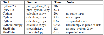
We start with the original pure_python.py code which has too many dereference operations. Running it with PyPy and no modifications results in an easily won speed-up.

Next we modify the code to make pure_python_2.py with less dereferences, it runs faster for both CPython and PyPy. Compiling with Cython doesn’t give us much compared to using PyPy but once we’ve added static types and expanded the complex arithmetic we’re down to 0.6s.
Cython with numpy vectors in place of list containers runs even faster (I’ve not drilled into this code to confirm if code differences can be attributed to this speed-up - perhaps this is an exercise for the reader?). Using ShedSkin with no code modificatoins we drop to 12s, after expanding the complex arithmetic it drops to 0.4s beating all the other variants.
Be aware that on my MacBook Cython uses gcc 4.0 and ShedSkin uses gcc 4.2 - it is possible that the minor speed variations can be attributed to the differences in compiler versions. I’d welcome someone with more time per- forming a strict comparison between the two versions (the 0.6s, 0.49s and 0.4s results) to see if Cython and ShedSkin are producing equivalently fast code.
Do remember that more manual work goes into creating the Cython version than the ShedSkin version.

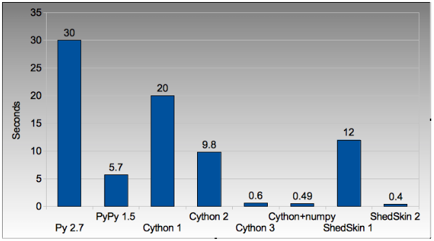
Compare CPython with PyPy and the improvements using Cython and ShedSkin here:

Figure 4.1: Run times on laptop for Python/C implementations
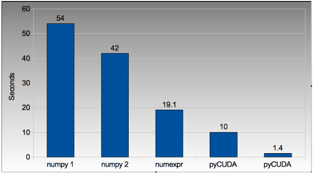
Next we switch to vector techniques for solving this problem. This is a less efficient way of tackling the problem as we can’t exit the inner-most loops early, so we do lots of extra work. For this reason it isn’t fair to compare this approach to the previous table. Results within the table however can be compared.
numpy_vector.py uses a straight-forward vector implementation. numpy_vector_2.py uses smaller vectors that fit into the MacBook’s cache, so less memory thrashing occurs. The numexpr version auto-tunes and auto- vectorises the numpy_vector.py code to beat my hand-tuned version.
The pyCUDA variants show a numpy-like syntax and then switch to a lower level C implementation. Note that the 9400M is restricted to single precision (float32) floating point operations (it can’t do float64 arithmetic like the rest of the examples), see the GTX 480 result further below for a float64 true comparison.
Even with a slow GPU you can achieve a nice speed improvement using pyCUDA with numpy-like syntax compared to executing on the CPU (admittedly you’re restricted to float32 math on older GPUs). If you’re prepared to recode the core bottleneck with some C then the improvements are even greater.

The reduction in run time as we move from CPU to GPU is rather obvious:

Figure 4.2: Run times on laptop using the vector approach
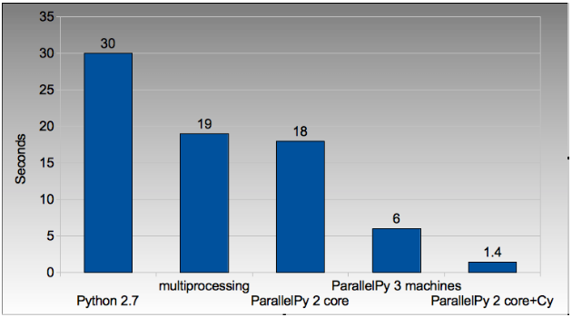
Finally we look at using multi-CPU and multi-computer scaling approaches. The goal here is to look at easy ways of parallelising to all the resources available around one desk (we’re avoiding large clusters and cloud solutions in this report).
The first result is the pure_python_2.py result from the second table (shown only for reference). multi.py uses the multiprocessing module to parallelise across two cores in my MacBook. The first ParallelPython example works exaclty the same as multi.py but has lower overhead (I believe it does less serialising of the environment). The second version is parallelised across three machines and their CPUs.
The final result uses the 0.6s Cython version (running on one core) and shows the overheads of splitting work and serialising it to new environments (though on a larger problem the overheads would shrink in comparison to the savings made).

The approximate halving in run-time is more visible in the figure below, in particular compare the last column with Cython 3 to the results two figures back.

Figure 4.3: Run times on laptop using multi-core approaches
4.2 2.9GHz i3 desktop with GTX 480 GPU
Here I’ve run the same examples on a desktop with a GTX 480 GPU which is far more powerful than my laptop’s 9400M, it can


