Using texture images
14.3 Texture and multiple levels of detail
14.5 Using transparent geometry with transparent texture images
14.6 Animated (video) texture mapping
The process of applying a bitmap to geometry is called texture mapping and is often a highly effective way of achieving apparent scene complexity while still using a relatively modest number of vertices. By the end of this chapter, you should be able to generate texture coordinates and apply a texture image to your geometry (e.g., figure 14.1).
If you are familiar with the process of texture mapping and texture coordinates, you may want to skim the first few sections and jump straight to the specifics of the Java 3D implementation.
As colors can only be associated with vertices in the model, if texture mapping was not used, a vertex would have to be located at every significant surface color transition. For highly textured surfaces such as wood or stone, this would quickly dominate the positions of the vertices rather than the geometric shape of the object itself. By applying an image to the geometric model, the apparent complexity of the model is increased while preserving the function of vertices for specifying relative geometry within the model.
Modern 3D computer games have used texture mapping extensively for a number of years, and first-person-perspective games such as Quake by Id software immerses the user in a richly texture-mapped world.
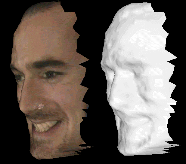
Figure 14.1 By applying a bitmap to the geometric model (left), very realistic results can be achieved even with a fairly coarse geometric mesh
Texture mapping is exactly what it says. As an application developer, you are defining a mapping from 3D coordinates into texture coordinates. Usually this equates to defining a coordinate mapping to go from a vertex’s 3D coordinates to a 2D pixel location within an image.
Defining coordinate mappings sounds pretty complicated, but in practice it can be as simple as saying the vertex located at position (1,1,1) should use the pixel located at (20,30) in the image named texture.jpg.
Looking at figure 14.2 it should be obvious that the renderer does some pretty clever stuff when it maps a texture onto a geometric model. The texture used was 64 x 64 pixels in size, but when it was rendered, the faces of each cube were about 200 x 200 pixels. So, the renderer had to resize the texture image on the fly to fit the face of each cube. Even tougher, you can see that what started out as a square texture image turned into a parallelogram as perspective and rotation were applied to the cube.
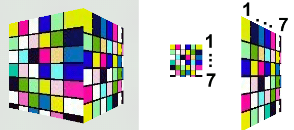
Figure 14.2 A texture-mapped cube (left); the texture image, actual size (middle); and the how the texture image was mapped onto one of the faces of the cube (right)
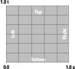
Figure 14.3 Texture coordinates range from 0.0 to 1.0 with the origin at the bottom left of the texture image. The horizontal dimension is commonly called s and the vertical dimension is called t
You should also be able to see that as the texture has been enlarged it has become pixilated. This is because several eventual screen pixels are all mapped to the same pixel within the texture image. This is a common problem with texture mapping and is visible in texture-mapped games such as Quake, as well.
To discuss the details of mapping between 3D vertex coordinates and texture pixels, some terminology must be introduced. Figure 14.3 illustrates texture coordinates. Instead of mapping to pixel locations directly (which would be relative to the size of the texture image), we use texture coordinates. Texture coordinates range from 0.0 to 1.0 in each dimension, regardless of the size of the image. We know therefore that the coordinates s = 0.5, t = 0.25 are always located halfway across the image and three-quarters of the way down from the top of the image. Note that the origin of the texture coordinate system is at the bottom left of the image, in contrast to many windowing systems that define the origin at the top left.
A pixel within an image that is used for texture mapping is often referred to as a texel.
There are essentially two types of texture mapping, static and dynamic. Defining a static mapping is the most commonly used and easiest form of texture mapping and is the subject of section 14.1.1.
14.1.1 Static mapping using per-vertex texture coordinates
Static mapping defines a static relationship between vertex coordinates and texture coordinates. This is usually implemented by simply assigning a texture coordinate to each vertex in the model (table 14.1).
Table 14.1 Static mapping
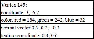
Vertex 143 has been assigned a number of attributes: coordinate (position), color, normal vector, and a texture coordinate.
The TextureTest example that follows can be used to experiment with the relationship among images, texture coordinates, and 3D vertex coordinates (figure 14.4).
TextureTest loads the following information from a simple ASCII text file:
For example, the data for the image in figure 14.4 is shown in table 14.2.
Table 14.2 Static mapping
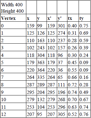
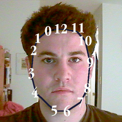
Figure 14.4 The TextureTest example loads an image and a list of texture coordinates and displays a portion of the image in a 3D scene by texture mapping it onto a TriangleArray
daniel.gif (name of the image file)
5 (size in the x direction)
1.0 (y scale factor)
13 (number of texture coordinates)
0.40 0.75 (texture coordinate 1, x y)
0.31 0.69
0.28 0.59
0.26 0.39
0.30 0.24
0.45 0.09
0.55 0.09
0.66 0.16
0.72 0.28
0.74 0.49
0.70 0.67
0.63 0.74
0.52 0.76 (texture coordinate 13, x y)
The Microsoft Excel spread sheet file daniel coords.xls with the TextureTest example contains the formulae necessary for the coordinate transformation (figure 14.5).
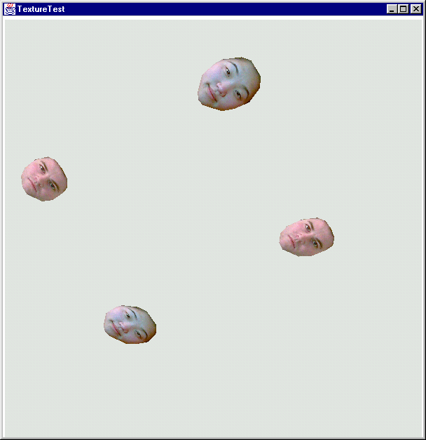
Figure 14.5 The TextureTest example in action. Four texture-mapped TriangleArrays have been created from two sets of texture coordinate data and images. The TriangleArrays are rotated using an Interpolator
IMPORTANT
The texture coordinates are specified in counterclockwise order. This is a requirement imposed by the com.sun.j3d.utils.geometry.Triangulator utility, which converts the polygon created from the texture coordinates into a TriangleArray.
The createTextureGeometry method performs most of the work related to assigning texture coordinates to vertices. There are eight basic steps:
1. Read Texture coordinates from file.
2. Generate vertex coordinates based on scaling and translating texture coordinates.
3. Load the texture image using the com.sun.j3d.utils.image.TextureLoader class and assign to an Appearance.
//load the texture image and assign to the appearance TextureLoader texLoader = new TextureLoader( texInfo.m_szImage,
Texture.RGB, this );
Texture tex = texLoader.getTexture();
app.setTexture( tex );
4. Create a GeometryInfo object to store the texture and vertex coordinates (POYGON_ARRAY).
//create a GeometryInfo for the QuadArray that was populated.
GeometryInfo gi = new GeometryInfo( GeometryInfo.POLYGON_ARRAY );
5. Assign the texture and vertex coordinates to the GeometryInfo object.
//assign coordinates
gi.setCoordinates( texInfo.m_CoordArray );
gi.setTextureCoordinates( texInfo.m_TexCoordArray );
6. Triangulate the GeometryInfo object.
//use the triangulator utility to triangulate the polygon
int[] stripCountArray = {texInfo.m_CoordArray.length};
int[] countourCountArray = {stripCountArray.length};
gi.setContourCounts( countourCountArray );
gi.setStripCounts( stripCountArray );
Triangulator triangulator = new Triangulator();
triangulator.triangulate( gi );
7. Generate Normal vectors for the GeometryInfo object.
//generate normal vectors for the triangles,
//not strictly necessary as we are not lighting the scene
//but generally useful
NormalGenerator normalGenerator = new NormalGenerator();
normalGenerator.generateNormals( gi );
8. Create a Shape3D object based on the GeometryInfo object.
//wrap the GeometryArray in a Shape3D and assign appearance
new Shape3D( gi.getGeometryArray(), app );
Please refer to TextureTest.java for the full example. The important methods are listed in full next.
//create a TransformGroup, position it, and add the texture
//geometry as a child node
protected TransformGroup createTextureGroup( String szFile,
double x, double y, double z, boolean bWireframe )
{
TransformGroup tg = new TransformGroup();
Transform3D t3d = new Transform3D();
t3d.setTranslation( new Vector3d( x,y,z ) );
tg.setTransform( t3d );
Shape3D texShape = createTextureGeometry( szFile, bWireframe );
if( texShape != null )
tg.addChild( texShape );
return tg;
}
//return a Shape3D that is a triangulated texture-mapped polygon
//based on the texture coordinates and name of texture image in the
//input file
protected Shape3D createTextureGeometry( String szFile, boolean bWireframe )
{
//load all the texture data from the file and
//create the geometry coordinates
TextureGeometryInfo texInfo = createTextureCoordinates(
szFile );
if( texInfo == null )
{
System.err.println( "Could not load texture info for file:" +
szFile );
return null;
}
//print some stats on the loaded file
System.out.println( "Loaded File: " + szFile );
System.out.println( " Texture image: " + texInfo.m_szImage );
System.out.println( " Texture coordinates: " +
texInfo.m_TexCoordArray.length );
//create an Appearance and assign a Material
Appearance app = new Appearance();
PolygonAttributes polyAttribs = null;
//create the PolygonAttributes and attach to the Appearance,
//note that we use CULL_NONE so that the "rear" side
//of the geometry is visible with the applied texture image
if( bWireframe == false )
{
polyAttribs = new PolygonAttributes(
PolygonAttributes.POLYGON_FILL,
PolygonAttributes.CULL_NONE, 0 );
}
else
{
polyAttribs = new PolygonAttributes(
PolygonAttributes.POLYGON_LINE,
PolygonAttributes.CULL_NONE, 0 );
}
app.setPolygonAttributes( polyAttribs );
//load the texture image and assign to the appearance
TextureLoader texLoader = new TextureLoader( texInfo.m_szImage,
Texture.RGB, this );
Texture tex = texLoader.getTexture();
app.setTexture( tex );
//create a GeometryInfo for the QuadArray that was populated.
GeometryInfo gi = new GeometryInfo( GeometryInfo.POLYGON_ARRAY
);
gi.setCoordinates( texInfo.m_CoordArray );
gi.setTextureCoordinates( texInfo.m_TexCoordArray );
//use the triangulator utility to triangulate the polygon
int[] stripCountArray = {texInfo.m_CoordArray.length};
int[] countourCountArray = {stripCountArray.length};
gi.setContourCounts( countourCountArray );
gi.setStripCounts( stripCountArray );
Triangulator triangulator = new Triangulator();
triangulator.triangulate( gi );
//Generate normal vectors for the triangles, not strictly
necessary
//as we are not lighting the scene, but generally useful.
NormalGenerator normalGenerator = new NormalGenerator();
normalGenerator.generateNormals( gi );
//wrap the GeometryArray in a Shape3D and assign appearance
return new Shape3D( gi.getGeometryArray(), app );
}
/*
* Handle the nitty-gritty details of loading the input file
* and reading (in order):
* - texture file image name
* - size of the geometry in the X direction
* - Y direction scale factor
* - number of texture coordinates
* - each texture coordinate (X Y)
* This could all be easily accomplished using a scenegraph
loader,
* but this simple code is included for reference.
*/
protected TextureGeometryInfo createTextureCoordinates( String szFile )
{
//create a simple wrapper class to package our return values
TextureGeometryInfo texInfo = new TextureGeometryInfo();
//allocate a temporary buffer to store the input file
StringBuffer szBufferData = new StringBuffer();
float sizeGeometryX = 0;
float factorY = 1;
int nNumPoints = 0;
Point2f boundsPoint = new Point2f();
try
{
//attach a reader to the input file
FileReader fileIn = new FileReader( szFile );
int nChar = 0;
//read the entire file into the StringBuffer while( true )
{
nChar = fileIn.read();
//if we have not hit the end of file
//add the character to the StringBuffer
if( nChar != -1 )
szBufferData.append( (char) nChar );
else
//hit EOF
break;
}
//create a tokenizer to tokenize the input file at whitespace
java.util.StringTokenizer tokenizer =
new java.util.StringTokenizer( szBufferData.toString() );
//read the name of the texture image
texInfo.m_szImage = tokenizer.nextToken();
//read the size of the generated geometry in the X dimension
sizeGeometryX = Float.parseFloat( tokenizer.nextToken() );
//read the Y scale factor
factorY = Float.parseFloat( tokenizer.nextToken() );
//read the number of texture coordinates
nNumPoints = Integer.parseInt( tokenizer.nextToken() );
//read each texture coordinate
texInfo.m_TexCoordArray = new Point2f[nNumPoints];
Point2f texPoint2f = null;
for( int n = 0; n < nNumPoints; n++ )
{
texPoint2f = new Point2f( Float.parseFloat(
tokenizer.nextToken() ),
Float.parseFloat( tokenizer.nextToken() ) );
texInfo.m_TexCoordArray[n] = texPoint2f;
//keep an eye on the extents of the texture coordinates
// so we can automatically center the geometry
if( n == 0 || texPoint2f.x > boundsPoint.x )
boundsPoint.x = texPoint2f.x;
if( n == 0 || texPoint2f.y > boundsPoint.y )
boundsPoint.y = texPoint2f.y;
}
}
catch( Exception e )
{
System.err.println( e.toString() );
return null;
}
//build the array of coordinates
texInfo.m_CoordArray = new Point3f[nNumPoints];
for( int n = 0; n < nNumPoints; n++ )
{
//scale and center the geometry based on the texture
Coordinates
texInfo.m_CoordArray[n] = new Point3f( sizeGeometryX *
texInfo.m_TexCoordArray[n].x - boundsPoint.x/2),
factorY * sizeGeometryX *
(texInfo.m_TexCoordArray[n].y - boundsPoint.y/2), 0 );
}
return texInfo;
}
As the TextureTest example illustrates, using a static mapping from vertex coordinates is relatively straightforward. Texture coordinates are assigned to each vertex, much like vertex coordinates or per-vertex colors. The renderer will take care of all the messy details of interpolating the texture image between projected vertex coordinates using projection and sampling algorithms.
Texture coordinates themselves are usually manually calculated or are the product of an automated texture-mapping process (such as 3D model capture or model editor).
Note that although we have called this section static mapping, there is nothing to prevent you from modifying the texture coordinates within a GeometryArray at runtime. Very interesting dynamic effects can be achieved through reassigning texture coordinates.
Care must be taken to ensure that texture images do not become too pixilated as they become enlarged and stretched by the sampling algorithm. The MIPMAP technique covered in detail in Section 14.3.4 is useful in this regard in that different sizes of different texture images can be specified.
Needless to say, texture images consume memory, and using large 24-bit texture images is an easy way to place a heavy strain on the renderer and push up total memory footprint. Of course, the larger the texture image, the less susceptible it is to becoming pixilated so a comfortable balance must be found between rendering quality, rendering speed, and memory footprint. You should also be very aware that different 3D rendering hardware performs texture mapping in hardware only if the texture image falls within certain criteria. Modern 3D rendering cards typically have 16 MB or more of texture memory, and 64 MB is now not uncommon. Most rendering hardware will render texture images of up to 512 x 512 pixels. You should consult the documentation for the 3D rendering cards that your application considers important.
14.1.2 Dynamic mapping using TexCoordGeneration
In contrast to a hard-coded static mapping between vertex coordinates and texture coordinates, dynamic texture mapping enables the application developer to define a mapping that is resolved by the renderer at runtime. Dynamic mapping is fairly unusual but is very useful for certain scientific visualization applications—where the position of a vertex in 3D space should correlate with its texture coordinate.
Rather than having to manually update the texture coordinate whenever a vertex moves, the application developer defines a series of planes that the renderer uses to calculate a texture coordinate.
The TexCoordTest example application explores the three texture coordinate generation options in Java 3D. These are TexCoordGeneration.EYE_LINEAR, TexCoordGeneration.OBJECT_LINEAR, and TexCoordGeneration.SPHERE_MAP (figures 14.6–14.11). Each will be described in turn in the sections that follow.

Figure 14.6 The TexCoordTest example application in action. The vertices in the undulating landscape do not have assigned texture coordinates, but rather a TexCoordGeneration object is used to calculate texture coordinates dynamically
OBJECT_LINEAR mode
The OBJECT_LINEAR texture coordinate generation mode calculates texture coordinates based on the relative positions of vertices. The TexCoordTest example creates a simulated landscape that has contours automatically mapped onto the landscape Everything above the y = 0 plane is texture-mapped green, while everything below is texture-mapped blue.
Figure 14.7 illustrates the texture image used in the TexCoordTest example for dynamic texture mapping. The texture image is 64 x 64 pixels and merely contains a single row of pixels that is of interest—the rest of the image is ignored. The bottom row of the image (t = 0) defines the colors to be dynamically applied to the landscape. The midpoint of the row (s = 0.5) defines the elevation = 0 (sea level) contour, while everything to the left of the midpoint is used for elevations below sea level, and everything to the right is used for elevations above sea level. Different colored pixels for contours are evenly spaced from the midpoint.
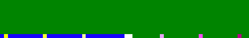
Figure 14.7 The texture image used to perform dynamic mapping of texture coordinates in the TexCoordTest example application
To map contours onto the landscape we merely need to define a mapping from the y coordinate of the landscape to the s coordinate of the texture image. That is, we are defining a 1D-to-1D mapping from vertex coordinates to texture coordi