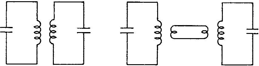
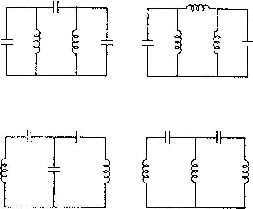
Radio signals carrying intelligence occupy a band of frequencies and circuits must be able to accept the whole of that band whilst rejecting all others. When tuned circuits are coupled together in the correct manner they form such a band-pass circuit. The coupling may be either by mutual inductance between the two inductances of the circuits as in Figure 5.3 or through discrete electrical components as in Figure 5.4.
Mutual inductance can be defined in terms of the number of flux linkages in the second coil produced by unit current in the first coil. The relationship is:
flux linkages in 2nd coilM
=
produced by current in 1st coil× 10−8 current in 1st coil
L
 Link
Link(a) Capacitive (b) Inductive High impedance, ‘top’ coupling
C1C2C1C2
 L
Lwhere M = mutual inductance in henries. The e.m.f. induced in the secondary is e2=−jωMI1 where I1 is the primary current.
The maximum value of mutual inductance that can exist is√L1L2 and the ratio of the actual mutual inductance to the maximum is the coefficient of coupling, k:
k=
√
M L1L2
The maximum value of k is 1 and circuits with a k of 0.5 or greater are said to be close coupled. Loose coupling refers to a k of less than 0.5. An advantage of coupling using discrete components is that the coupling coefficient is more easily determined. Approximations for k for the coupling methods shown in Figure 5.4 are:
(a) k = √Cm where Cm is much smaller than (C1C2)C1C2√(b) kL1L2 where Lm is much larger than (L1L2) =Lm√
(c) kC1C2 where Cm is much larger than (C1C2) =Cm
(d) kLm where Lm is much smaller than (L1L2) = √L1L2
When two circuits tuned to the same frequency are coupled their mutual response curve takes the forms shown in Figure 5.5, the actual shape depending on the degree of coupling.
Secondary current
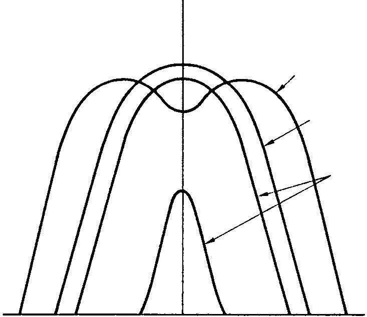 k= critical
When coupling is very loose the frequency response and the current in the primary circuit are very similar to that of the primary circuit alone. Under these conditions the secondary current is small and the secondary response curve approximates to the product of the responses of both circuits considered separately.
As coupling is increased the frequency response curves for both circuits widen and the secondary current increases. The degree of coupling where the secondary current attains its maximum possible value is called the critical coupling. At this point the curve of the primary circuit shows two peaks, and at higher coupling factors the secondary response also shows two peaks. The peaks become more prominent and further apart as coupling is increased, and the current at the centre frequency decreases.