pressure. Blue: simulation without optimization, red: Simulation with optimization.
4.4 Neural network controller
Optimization previously done "off line", would be directly unexploited "on-line" by a
controlling processor seen the enormous computation time that is necessary to resolve the
optimization problem. In order to integrate the results of this optimization’s procedure in a
closed loop controller (ref fig. 3), and to be able to use it in real time engine applications, we
suggest to use a black box model based on neurons. Neural network is a powerful tool
capable of simulating the engine’s optimal control variables with good precision and almost
instantly.
The neural network inputs are the fuel mass flow rate and the resistant torque, and its
output variables are the optimal values of the air mass flow rate and the intake pressure.
However in real time engine applications, the injected fuel flow rate is measurable, while the
resistant torque is not. Consequently, we suggest substituting this variable by the crankshaft
angular speed which can be easily measured and which is widely used in passenger cars
controlling systems.
Firstly, we need to create a large database which will be used to train the neural model, and
which covers all the functioning area of the engine in order to have a good precision and a
highly engine performance. The database is created using the optimization process as
explained in subsection 4.3.
Then we have to judicially choose the number of the inputs time sequence to be used, in
order to capture the inputs dynamic effects and accurately predict the output variables.
With intensive simulations and by trial and error, we find out that a neural network with
inputs the fuel mass flow rate and the crankshaft angular speed at instant (i), (i-1) and (i-2) is
capable of precisely predicting the optimal values of the air mass flow rate and the intake
Optimized Method for Real Time Nonlinear Control
183
pressure at current instant (i). Fig. 12 describes the neural network. The network is built
using one hidden layer and one output layer, the activation functions of the hidden layer are
sigmoid; the ones at the output layer are linear.
. m f ( i)
.
.
f
m ( i)
1
mc ( i)
.
f
m ( i )
2
.
.
(
w i)
p ( i)
.
c
(
w i )
1
.
.
(
w i 2)
Fig. 12. The structural design of the neural network adopted in this paper for predicting the
optimal control of the in-air filling and the intake pressure in real time applications.
The number of neurons in the hidden layer is determined by referring to the errors
percentage of the points which are under a certain reference value wisely chosen; the
errors percentage (table 3) are the results of the difference between the outputs of the
network after the training process is completed, and the desired values used in the training
database.
Table 3 shows the results of the neural networks with different number of neurons in their
hidden layer, these networks are trained with the same database until a mean relative error
equal to 10-8 is reached or maximum training time is consumed. The values in the table
represent the percentage of the neural network results respecting the specified error
percentage computed with respect to the reference values.
Error percentage
Number of neurons of the
Relative
hidden layer
< 10
< 1 % < 5 %
error
%
110 57.71
88.85 96.71 3.6 10-5
120 98.428
100
100
10-8
130 98.734
100
100
10-8
140 99
100
100
10-8
Table 3. Results of four neural networks trained using different neurons number in their
hidden layer and the same database.
The neural network adopted in this paper includes one hidden layer with 140 neurons and
one output layer with 2 neurons. Fig. 13 and 14 show a comparison between the air mass
flow rate and the intake pressure calculated using the theoretical optimization procedure,
and the ones computed using the neural network. The results are almost identical; the mean
relative error is 10-6.
184
Applications of Nonlinear Control
0.42
Optimization Process
Neural Model
0.4
2.46
2.44
0.38
ar]B 2.42
0.36
g/s]
re [
K [
2.4
C
ressu
m'
0.34
P
2.38
takeIn
0.32
2.36
0.3
Optimization Process
2.34
Neural Model
0.28
2.32
0
1
2
3
0
1
2
3
t [s]
t [s]
0.45
2.5
Optimization Process
Optimization Process
Neural Model
Neural Model
0.4
2.4
2.3
0.35
ar]B 2.2
0.3
/s]
[Kg
2.1
C
ressure [
m'
0.25
ke P
2
taIn
0.2
1.9
0.15
1.8
0.1
1.7
0
1
2
3
0
1
2
3
t [s]
t [s]
Fig. 13. & 14. Comparison between the neural network outputs and the optimal values of the
air mass flow rate and the intake pressure.
5. General conclusions
We successfully developed and validated a mean value physical model that describes the
gas states evolution and the opacity of a diesel engine with a variable geometry
turbocharger. Then we proposed a dynamic control based on the optimal “in-air cylinders
filling” in order to minimize the pollutants emissions while enhancing the engine
performance. The optimization process is described in detail and the simulation results (fig.
8-11) prove to be very promising. In addition, the control principle as described here with
the opacity criterion can be easily applied to other pollutants which have available physical
model. This will be the object of future publications.
Optimized Method for Real Time Nonlinear Control
185
Also, in order to overcome on line computation difficulties, a real time dynamic control based
on the neural network is suggested; therefore the optimal static maps of the fig. 2 can be
successfully replaced by dynamic maps simulated in real time engine functioning (fig. 15).
Xp
m'
GV
Opacity
C, ref
Neural
Network Pref
P.I
Engine
EGR
m’
P
C
Fig. 15. Proposed control in closed loop
Finally, we should note that, in this chapter, while we did find, in theory, the optimal air mass
flow rate and intake pressure necessary to minimize the opacity, but we didn’t discuss the
mechanical equipments required to provide the optimal intake pressure and intake air flow
rate in real time engine applications. The practical implementation of the dynamic control is an
important question to be studied thereafter. The use of a turbo-compressor with variable
geometry and/or with Waste-Gate, and/or electric compressor is to be considered.
6. References
Arnold, J.F. (2007). Proposition d’une stratégie de commande à base de logique floue pour la commande
du circuit d’air d’un moteur Diesel. PHD thesis, Rouen University, (March 2007), France.
Bai, L. & Yang, M. (2002). Coordinated control of EGR and VNT in turbocharged Diesel engine
based on intake air mass observer, SAE Technical paper 2002-01-1292, (March 2002).
Bartoloni, G. (1989). Chattering Phenomena in Discontinuous Control Systems. International
Journal on Systems Sciences, Vol. 20, Issue 12, (February 1989), ISSN 0020-7721.
Bellman, R. (1975). Dynamic programming. Princeton University Press, (1957), Princeton, NJ.
Doyle, J.C. (1979). Robustness of multiloop linear feedback systems” Proceedings of the 1978
IEEE Conference on Decision and Control, pages 12–18, Orlando, December 1979.
Dreyfus, S.E. (1962). Variational Problems with Inequality Constraints. Journal of
Mathematical Analysis and Applications, Vol. 4, Issue 2, (July 1962), ISSN 0022-247X.
Friedland, B. (1996). Advanced Control System Design. Prentice-Hall, Englewood Cliffs, ISBN
978-0130140104, NJ, 1996.
Hafner, M. (2000). A Neuro-Fuzzy Based Method for the Design of Combustion Engine
Dynamometer Experiments. SAE Technical Paper 2000-01-1262, (March 2000).
Hafner, M. (2001). Model based determination of dynamic engine control function
parameters. SAE Technical Paper 2001-01-1981, (May 2001).
Hahn, W. (1967). Stability of Motion, Springer-Verlag, ISBN 978-3540038290, New York, 1967.
Hassenfolder, M. & Gissinger, G.L. (1993). Graphical eider for modelling with bound graphs
in processes ». ICBGM’93, pp. 188-192, Californie, January 1993.
Jung, M. (2003). Mean value modelling and robust control of the airpath of a turbocharged diesel
engine. Thesis for doctor of philosophy, University of Cambridge, 2003.
Kao, M. & Moskwa, J.J. (1995). Turbocharger Diesel engine modelling for non linear engine
control and state estimation. Trans ASME, Journal of Dynamic Systems Measurement
and Control, Vol. 117, Issue 1, pp. 20-30, (March 1995), ISSN 0022-0434.
186
Applications of Nonlinear Control
Li, D.; Lu, D.; Kong X. & Wu G. (2005). Implicit curves and surfaces based on BP neural
network. Journal of Information & Computational Science, Vol. 2, No 2, pp. 259-271,
(2005), ISSN 1746-7659.
Minoux, M. (1983). Programmation Mathématique, Théorie et Algorithmes. tome 1 & 2, editions
dunod, ISBN 978-2743010003, Paris 1983.
Omran, R.; Younes, R. & Champoussin, J.C. (2008a). Optimization of the In-Air Cylinders
Filling for Emissions Reduction in Diesel engines, SAE Technical Paper 2008-01-1732,
(June 2008).
Omran, R. ; Younes, R. & Champoussin, J.C. (2008b). Neural Networks for Real Time non
linear Control of a Variable Geometry Turbocharged Diesel Engine , International
Journal of Robust and non Linear Control, Vol. 18, Issue 12, pp. 1209-1229, (August
2008), ISSN 1099-1239.
Ouenou-Gamo, S. (2001). Modélisation d’un moteur Diesel suralimenté, PHD Thesis, Picardie
Jules Vernes University, (2001), France.
Ouladssine, M.; Blosh, G. & Dovifazz X. (2004). Neural Modeling and Control of a Diesel
Engine with Pollution Constraints . Journal of Intelligent and Robotic Systems; Theory
and Application, Vol. 41, Issue 2-3, (January 2005), ISSN 0921-0296.
Outbib, R. & Vivalda, J.C. (1999). A note on Feedback stabilization of smooth nonlinear
systems. IEEE Transactions on Automatic Control. Vol. 44, No 1, pp. 200-203, (August
1999), ISSN 0018-9286.
Outbib, R. & Richard, E. (2000). State Feedback Stabilization of an Electropneumatic System.
ASME Journal of Dynamic Systems Measurement and Control. Vol. 122, pp 410-415,
(September 2000), ISSN 0022-0434.
Outbib, R. & Zasadzinski, M. (2009). Sliding Modes Control, In: Control Methods for Electrical
Machines, René Husson Editor, Ch. 6, pp. 169-204, 2009. Wiley, ISBN 978-1-84821-
093-6, USA.
Pontryagin, L.S.; Boltyanskii, V.; Gamkrelidze, R.V & Mishchenko, E.F. (1962). The
Mathematical Theory of Optimal Processes. 1962, John Wiley & Sons, USA
Rivals, I. (1995). Modélisation et commande de processus par réseaux de neurones ; application au
pilotage d’un véhicule autonome, PHD Thesis, Paris 6 University, (1995), France.
Sira-Ramirez, H. (1987). Differential Geometric Methods in Variable-Structure Control.
International Journal of Control, Vol. 48, Issue 2, (March 1987), pp. 1359-1390, ISSN
0020-7179.
Slotine, J-J.E. (1984). Sliding Controller Design for Non-linear System. International Journal of
Control, Vol. 40, Issue 2, pp. 421-434, (March 1984), ISSN 0020-7179.
Utkin, V.I. (1992). Sliding Modes in Control and Optimization, Springer-Verlag, ISBN 978-
0387535166, Berlin 1992.
Winterbonne, D.E. & Horlock, J.H. (1984). The thermodynamics and gas dynamics internal
combustion engines. Oxford Science Publication, ISBN 978-0198562122, London 1984.
Younes, R. (1993). Elaboration d’un modèle de connaissance du moteur diesel avec
turbocompresseur à géométrie variable en vue de l’optimisation de ses émissions. PHD
Thesis, Ecole Centrale de Lyon, (November 1993), France.
Zames, G. (1981). Feedback and optimal sensitivity: Model reference transformations,
multiplicative seminorms, and approximative inverse” IEEE Transcations on
Automatic Control, Vol. 26, Issue 2, pp. 301–320, (June 1981), ISSN 0018-9286.
Zweiri Y.H. (2006). Diesel engine indicated torque estimation based on artificial neural
networks. International Journal of Intelligent Technology, Vol. 1, No 1, pp. 233-239,
(July 2006), ISSN 1305-6417.
0
11
Nonlinear Phenomena and Stability Analysis for
Discrete Control Systems
Yoshifumi Okuyama
Tottori University, Emeritus
Japan
1. Introduction
Almost all feedback control systems are realized using discretized (discrete-time and
discrete-value, i.e., digital) signals.
However, the analysis and design method of
discretized/quantized (nonlinear) control systems has not been established (Desoer et al.,
1975; Elia et al., 2001; Harris et al., 1983; Kalman, 1956; Katz, 1981). This article analyzes
the nonlinear phenomena and stability of discretized control systems in a frequency domain1
(Okuyama, 2006; 2007; 2008).
In these studies, it is assumed that the discretization is
executed on the input and output sides of a nonlinear element at equal spaces, and the
sampling period is chosen of such a size suitable for the discretization in the space. Based
on the premise, the discretized (point-to-point) nonlinear characteristic is examined from two
viewpoints, i.e., global and local. By partitioning the discretized nonlinear characteristic into
two sections and by defining a sectorial area over a specified threshold, the concept of the
robust stability condition for nonlinear discrete-time systems is applied to the discretized
(hereafter, simply wrriten as discrete) nonlinear control system in question. As a result, the
nonlinear phenomena of discrete control systems are clarified, and the stability of discrete
nonlinear feedback systems is elucidated.
h
r† ✲+ ❣ e ✲
†
v
N( e†)
✟❆❯
DH
✻
−
S1
h
y†
u
❄+ d
DH
❍
✁☛
G( s)
✛
❣✛+
S2
Fig. 1. Nonlinear sampled-data control system.
2. Discrete nonlinear control system
The discrete nonlinear control system to be considered here is represented by a sampled-data
control system with two samplers, S1, S2 and the continuous nonlinear characteristic N( ·) as
1 In the time domain analysis (e.g., Lyapunov function method), it is difficult to find a Lyapunov function
for the discretized (severe nonlinear characteristic) feedback system. The frequency domain analysis
will be important in cases where physical systems with uncertainty in the system-order are considered.
188
2
Nonlinear Control
Applications of Nonlinear Control
Nd( e)
r ✲+ ❣ e ✲ D ✲
e†
✲
v†
v
1
N( e†)
D 2
✻
−
y
u†
❄+ d†
G( z)
✛
❣✛+
Fig. 2. Discrete nonlinear control system.
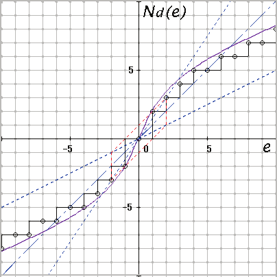
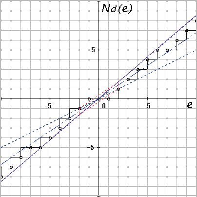
(a)
(b)
Fig. 3. Discretized nonlinear characteristics.
shown in Fig. 1. Here, DH denotes the discretization and zero-order-hold, which are usually
performed in A/D(D/A) conversion, and G( s) is the transfer function of the linear controlled
system. It is assumed that the two samplers with a sampling period h operate synchronously.
The sampled-data control system can be equivalently transformed into a discrete control
system as shown in Fig. 2. Here, G( z) is the z-transform of G( s) together with zero-order-hold, and D 1 and D 2 are the discretizing units on the input and output sides of the nonlinear
element, respectively. The relationship between e and v† = Nd( e) in the figure becomes a
stepwise nonlinear characteristic on integer grid coordinates as shown in Fig. 3 (a). Here, a
round-down discretization, which is usually executed on a computer, is applied. Therefore,
the relationship between e† and u† is indicated by small circles (i.e. a point-to-point transition)
on the stepwise nonlinear characteristic. Even if continuous characteristic N( ·) is linear, the
discretized characteristic v† becomes nonlinear on integer grid coordinates as shown in Fig. 3
(b) (Okuyama, 2009).
In Fig. 2, each symbol e, u, y, · · · indicates the sequence e( k), u( k), y( k), · · · , ( k = 0, 1, 2, · · · ) in discrete time, but for continuous value. On the other hand, each symbol e†, u†, · · · indicates a
Nonlinear Phenomena and Stability Analysis for Discrete Control Systems
189
Nonlinear Phenomena and Stability Analysis for Discrete Control Systems
3
discrete value that can be assigned to an integer number, e.g.,
e† ∈ {· · · , − 3 γ, − 2 γ, −γ, 0, γ, 2 γ, 3 γ, · · · }, u† ∈ {· · · , − 3 γ, − 2 γ, −γ, 0, γ, 2 γ, 3 γ, · · · }, where γ is the resolution of each variable. Here, it is assumed that the input and output signals
of the nonlinear characteristic have the same resolution in the discretization. In the figure,
e† and u† also represent the sequence e†( k) and u†( k). Without loss of generality, hereafter, γ = 1.0 is assumed. Thus, the input and output variables of the nonlinear element can be
considered in the set of integer numbers, i.e.,
e†( k), u†( k) ∈ Z
def
Z = {· · · , − 3, − 2, − 1, 0, 1, 2, 3, · · · }.
3. Equivalent discrete-time system
In this study, the stepwise and point-to-point nonlinear characteristic is partitioned into the
following two sections:
Nd( e) = K( e + ν( e)), 0 < K < ∞,
|ν( e) | ≤ ¯ ν < ∞,
(1)
for |e| < ε, and
Nd( e) = K( e + n( e)), 0 < K < ∞,
|n( e) | ≤ α|e|, 0 < α ≤ 1,
(2)
for |e| ≥ ε, where ν( e) and n( e) are nonlinear terms relative to nominal line