View1
by Markus Pueschel, Carnegie Mellon University
In infinite, or non-periodic, discrete-time signal processing, there is
a strong connection between the z-transform, Laurent series, con-
volution, and the discrete-time Fourier transform (DTFT) [277].
As one may expect, a similar connection exists for the DFT but
bears surprises. Namely, it turns out that the proper framework
for the DFT requires modulo operations of polynomials, which
means working with so-called polynomial algebras [138]. Asso-
ciated with polynomial algebras is the Chinese remainder theo-
rem, which describes the DFT algebraically and can be used as
a tool to concisely derive various FFTs as well as convolution al-
gorithms [268], [409], [414], [12] (see also Winograd’s Short DFT
Algorithms (Chapter 7)). The polynomial algebra framework was
fully developed for signal processing as part of the algebraic sig-
nal processing theory (ASP). ASP identifies the structure under-
lying many transforms used in signal processing, provides deep
insight into their properties, and enables the derivation of their fast
1This content is available online at <http://cnx.org/content/m16331/1.14/>.
Available for free at Connexions
<http://cnx.org/content/col10683/1.5>
89
CHAPTER 8. DFT AND FFT: AN
90
ALGEBRAIC VIEW
algorithms [295], [293], [291], [294]. Here we focus on the alge-
braic description of the DFT and on the algebraic derivation of the
general-radix Cooley-Tukey FFT from Factoring the Signal Pro-
cessing Operators (Chapter 6). The derivation will make use of
and extend the Polynomial Description of Signals (Chapter 4). We
start with motivating the appearance of modulo operations.
The z-transform associates with infinite discrete signals X =
(· · · , x (−1) , x (0) , x (1) , · · · ) a Laurent series:
X → X (s) = ∑ x(n)sn.
(8.1)
n∈Z
Here we used s = z−1 to simplify the notation in the following.
The DTFT of X is the evaluation of X (s) on the unit circle
X e− jω ,
− π < ω ≤ π.
(8.2)
Finally, filtering or (linear) convolution is simply the multiplica-
tion of Laurent series,
H ∗ X ↔ H (s) X (s) .
(8.3)
For finite signals X = (x (0) , · · · , x (N − 1)) one expects that the
equivalent of (8.1) becomes a mapping to polynomials of degree
N − 1,
N−1
X → X (s) = ∑ x(n)sn,
(8.4)
n=0
and that the DFT is an evaluation of these polynomials. Indeed,
the definition of the DFT in Winograd’s Short DFT Algorithms
(Chapter 7) shows that
C (k) = X W k
N
= X e− j 2πk
N
,
0 ≤ k < N,
(8.5)
i.e., the DFT computes the evaluations of the polynomial X (s) at
the nth roots of unity.
Available for free at Connexions
<http://cnx.org/content/col10683/1.5>
91
The problem arises with the equivalent of (8.3), since the multipli-
cation H (s) X (s) of two polynomials of degree N − 1 yields one of
degree 2N − 2. Also, it does not coincide with the circular convo-
lution known to be associated with the DFT. The solution to both
problems is to reduce the product modulo sn − 1:
H∗circX ↔ H (s) X (s) mod (sn − 1) .
(8.6)
Concept
Infinite Time
Finite Time
Signal
X (s)
=
N−1
∑
x (n) sn
n=0
∑n∈ x (n) sn
Z
Filter
H (s)
=
N−1
∑
h (n) sn
n=0
∑n∈ h (n) sn
Z
Convolution
H (s) X (s)
H (s) X (s) mod (sn − 1)
Fourier transform
DTFT: X e− jω ,
−DFT: X e− j 2πk
n
,
0 ≤
π < ω ≤ π
k < n
Table 8.1: Infinite and finite discrete time signal processing.
The resulting polynomial then has again degree N − 1 and this form
of convolution becomes equivalent to circular convolution of the
polynomial coefficients. We also observe that the evaluation points
in (8.5) are precisely the roots of sn − 1. This connection will be-
come clear in this chapter.
The discussion is summarized in Table 8.1.
The proper framework to describe the multiplication of polynomi-
als modulo a fixed polynomial are polynomial algebras. Together
with the Chinese remainder theorem, they provide the theoretical
underpinning for the DFT and the Cooley-Tukey FFT.
Available for free at Connexions
<http://cnx.org/content/col10683/1.5>
CHAPTER 8. DFT AND FFT: AN
92
ALGEBRAIC VIEW
In this chapter, the DFT will naturally arise as a linear mapping
with respect to chosen bases, i.e., as a matrix. Indeed, the def-
inition shows that if all input and outputs are collected into vec-
tors X = (X (0) , · · · , X (N − 1)) and C = (C (0) , · · ·C (N − 1)), then
Winograd’s Short DFT Algorithms (Chapter 7) is equivalent to
C = DFT NX,
(8.7)
where
DFT N = W kn
N
.
(8.8)
0≤k,n<N
The matrix point of view is adopted in the FFT books [388], [381].
8.1 Polynomial Algebras and the DFT
In this section we introduce polynomial algebras and explain how
they are associated to transforms. Then we identify this connec-
tion for the DFT. Later we use polynomial algebras to derive the
Cooley-Tukey FFT.
For further background on the mathematics in this section and
polynomial algebras in particular, we refer to [138].
8.1.1 Polynomial Algebra
An algebra A is a vector space that also provides a multiplication
of its elements such that the distributivity law holds (see [138] for
a complete definition). Examples include the sets of complex or
real numbers C or R, and the sets of complex or real polynomials
in the variable s: C [s] or R [s].
The key player in this chapter is the polynomial algebra. Given a
Available for free at Connexions
<http://cnx.org/content/col10683/1.5>
93
fixed polynomial P (s) of degree deg (P) = N, we define a polyno-
mial algebra as the set
C [s] /P (s) = {X (s) | deg (X ) < deg (P)}
(8.9)
of polynomials of degree smaller than N with addition and mul-
tiplication modulo P. Viewed as a vector space, C [s] /P (s) hence
has dimension N.
Every polynomial X (s) ∈ C [s] is reduced to a unique polynomial
R (s) modulo P (s) of degree smaller than N. R (s) is computed
using division with rest, namely
X (s) = Q (s) P (s) + R (s) ,
deg (R) < deg (P) .
(8.10)
Regarding this equation modulo P, P (s) becomes zero, and we get
X (s) ≡ R (s) mod P (s) .
(8.11)
We read this equation as “X (s) is congruent (or equal) R (s) mod-
ulo P (s).” We will also write X (s) mod P (s) to denote that X (s)
is reduced modulo P (s). Obviously,
P (s) ≡ 0 mod P (s) .
(8.12)
As a simple example we consider A = C [s] / s2 − 1 , which has
dimension 2. A possible basis is b = (1, s). In A , for example,
s · (s + 1) = s2 + s ≡ s + 1 mod
s2 − 1 , obtained through division
with rest
s2 + s = 1 · s2 − 1 + (s + 1)
(8.13)
or simply by replacing s2 with 1 (since s2 − 1 = 0 implies s2 = 1).
8.1.2 Chinese Remainder Theorem (CRT)
Assume P (s) = Q (s) R (s) factors into two coprime (no common
factors) polynomials Q and R. Then the Chinese remainder theo-
Available for free at Connexions
<http://cnx.org/content/col10683/1.5>
CHAPTER 8. DFT AND FFT: AN
94
ALGEBRAIC VIEW
rem (CRT) for polynomials is the linear mapping2
∆
:
C [s] /P (s)
→
C [s] /Q (s)
⊕
(8.14)
C [s] /R (s) , X (s)
→
(X (s) mod Q (s) , X (s) mod R (s)) .
Here, ⊕ is the Cartesian product of vector spaces with elementwise
operation (also called outer direct sum). In words, the CRT asserts
that computing (addition, multiplication, scalar multiplication) in
C [s] /P (s) is equivalent to computing in parallel in C [s] /Q (s) and
C [s] /R (s).
If we choose bases b, c, d in the three polynomial algebras, then ∆
can be expressed as a matrix. As usual with linear mappings, this
matrix is obtained by mapping every element of b with ∆, express-
ing it in the concatenation c ∪ d of the bases c and d, and writing
the results into the columns of the matrix.
As an example, we consider again the polynomial P (s) = s2 − 1 =
(s − 1) (s + 1) and the CRT decomposition
∆ : C [s] / s2 − 1 → C [s] / (x − 1) ⊕ C [s] / (x + 1) .
(8.15)
As bases, we choose b = (1, x) , c = (1) , d = (1). ∆ (1) = (1, 1)
with the same coordinate vector in c ∪ d = (1, 1). Further, because
of x ≡ 1 mod (x − 1) and x ≡ −1 mod (x + 1), ∆ (x) = (x, x) ≡
(1, −1) with the same coordinate vector. Thus, ∆ in matrix form is
the so-called butterfly matrix, which is a DFT of size 2: DFT 2 =
1
1
.
1 −1
2More precisely, isomorphism of algebras or isomorphism of A -modules.
Available for free at Connexions
<http://cnx.org/content/col10683/1.5>
95
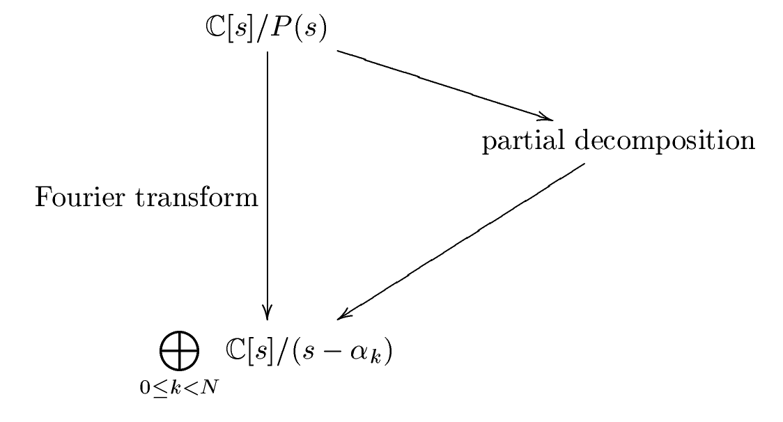
8.1.3 Polynomial Transforms
Assume
P (s) ∈ C [s] has pairwise distinct zeros α =
(α0, · · · , αN−1).
Then the CRT can be used to completely
decompose C [s] /P (s) into its spectrum:
∆
:
C [s] /P (s)
→
C [s] / (s − α0)
⊕
(8.16)
· · ·
⊕
C [s] / (s − αN−1) , X (s)
→
(X (s) mod (s − α0) , · · · , X (s) mod (s − αN−1)) =
(s (α0) , · · · , s (αN−1)) .
If we choose a basis b = (P0 (s) , · · · , PN−1 (s)) in C [s] /P (s) and
bases bi = (1) in each C [s] / (s − αi), then ∆, as a linear mapping,
is represented by a matrix. The matrix is obtained by mapping
every basis element Pn, 0 ≤ n < N, and collecting the results in the
columns of the matrix. The result is
Pb, = [P
(8.17)
α
n (αk)]0≤k,n<N
and is called the polynomial transform for A = C [s] /P (s) with
basis b.
If, in general, we choose bi = (βi) as spectral basis, then the matrix
corresponding to the decomposition (8.16) is the scaled polyno-
mial transform
diag0≤k<N (1/βn) Pb, ,
(8.18)
α
where diag0≤n<N (γn) denotes a diagonal matrix with diagonal en-
tries γn.
We jointly refer to polynomial transforms, scaled or not, as Fourier
transforms.
Available for free at Connexions
<http://cnx.org/content/col10683/1.5>
CHAPTER 8. DFT AND FFT: AN
96
ALGEBRAIC VIEW
8.1.4 DFT as a Polynomial Transform
We show that the DFT N is a polynomial transform for A =
C [s] / sN − 1 with basis b = 1, s, · · · , sN−1 . Namely,
sN − 1 = ∏
x − W k
N
,
(8.19)
0≤k<N
which means that ∆ takes the form
∆
:
C [s] / sN − 1
→ C [s] / s −W 0 ⊕
N
(8.20)
· · ·
⊕
C [s] / s − W N−1 , X (s)
→
N
X (s) mod s −W 0 , · · · , X (s) mod
s − W N−1
=
N
N
X W 0 , · · · , X W N−1
.
N
N
The associated polynomial transform hence becomes
Pb, = Wkn
= DFT
α
N
N .
(8.21)
0≤k,n<N
This interpretation of the DFT has been known at least since [409],
[268] and clarifies the connection between the evaluation points in
(8.5) and the circular convolution in (8.6).
In [40], DFTs of types 1–4 are defined, with type 1 being the stan-
dard DFT. In the algebraic framework, type 3 is obtained by choos-
ing A = C [s] / sN + 1 as algebra with the same basis as before:
P
(k+1/2)n
b,
= W
= DFT -3
α
N
N ,
(8.22)
0≤k,n<N
The DFTs of type 2 and 4 are scaled polynomial transforms [295].
Available for free at Connexions
<http://cnx.org/content/col10683/1.5>
97
8.2 Algebraic Derivation of the Cooley-
Tukey FFT
Knowing the polynomial algebra underlying the DFT enables us to
derive the Cooley-Tukey FFT algebraically. This means that in-
stead of manipulating the DFT definition, we manipulate the poly-
nomial algebra C [s] / sN − 1 . The basic idea is intuitive. We
showed that the DFT is the matrix representation of the complete
decomposition (8.20). The Cooley-Tukey FFT is now derived by
performing this decomposition in steps as shown in Figure 8.1.
Each step yields a sparse matrix; hence, the DFT N is factorized
into a product of sparse matrices, which will be the matrix repre-
sentation of the Cooley-Tukey FFT.
Figure 8.1: Basic idea behind the algebraic derivation of
Cooley-Tukey type algorithms
This stepwise decomposition can be formulated generically for
polynomial transforms [292], [294]. Here, we consider only the
DFT.
Available for free at Connexions
<http://cnx.org/content/col10683/1.5>
CHAPTER 8. DFT AND FFT: AN
98
ALGEBRAIC VIEW
We first introduce the matrix notation we will use and in particu-
lar the Kronecker product formalism that became mainstream for
FFTs in [388], [381].
Then we first derive the radix-2 FFT using a factorization of
sN − 1. Subsequently, we obtain the general-radix FFT using a
decomposition of sN − 1.
8.2.1 Matrix Notation
We denote the N × N identity matrix with IN, and diagonal matrices
with
γ0
. .
.
diag
0≤k<N (γk) =
.
(8.23)
γN−1
The N × N stride permutation matrix is defined for N = KM by
the permutation
LN
M : iK + j → jM + i
(8.24)
for 0 ≤ i < K, 0 ≤ j < M. This definition shows that LN trans-
M
poses a K × M matrix stored in row-major order. Alternatively, we
can write
LN : i → iM mod N − 1, for 0 ≤ i < N −
M
(8.25)
1, N − 1 → N − 1.
Available for free at Connexions
<http://cnx.org/content/col10683/1.5>
99
For example (· means 0),
1
·
·
·
·
·
·
· 1 ·
·
·
·
·
·
· 1 ·
L6 =
.
2
(8.26)
·
1
·
·
·
·
·
·
·
1
·
·
·
·
·
·
·
1
LN
is sometimes called the perfect shuffle.
N/2
Further, we use matrix operators; namely the direct sum
A
A ⊕ B =
(8.27)
B
and the Kronecker or tensor product
A ⊗ B = ak, B
,
for A = a
k,
k,
.
(8.28)
In particular,
A
. .
.
I
n ⊗ A = A ⊕ · · · ⊕ A =
(8.29)
A
is block-diagonal.
Available for free at Connexions
<http://cnx.org/content/col10683/1.5>
CHAPTER 8. DFT AND FFT: AN
100
ALGEBRAIC VIEW
We may also construct a larger matrix as a matrix of matrices, e.g.,
A B
.
(8.30)
B A
If an algorithm for a transform is given as a product of sparse
matrices built from the constructs above, then an algorithm for the
transpose or inverse of the transform can be readily derived using
mathematical properties including
(AB)T = BT AT ,
(AB)−1 = B−1A−1,
(A ⊕ B)T = AT ⊕ BT , (A ⊕ B)−1 = A−1 ⊕ B−1,
(8.31)
(A ⊗ B)T = AT ⊗ BT , (A ⊗ B)−1 = A−1 ⊗ B−1.
Permutation matrices are orthogonal, i.e., PT = P−1. The transpo-
sition or inversion of diagonal matrices is obvious.
8.2.2 Radix-2 FFT
The DFT decomposes A = C [s] / sN − 1
with basis b =
1, s, · · · , sN−1 as shown in (8.20). We assume N = 2M. Then
s2M − 1 = sM − 1
sM + 1
(8.32)
factors and we can apply the CRT in the following steps:
C [s] / sN − 1
(8.33)
→ C [s] / sM − 1 ⊕ C [s] / sM + 1
→
⊕ C [s] / x −W 2i ⊕ ⊕
N
C [s] / x − W 2i+1
M
0≤i<M
0≤i<M
(8.34)
→
⊕ C [s] / x −W i .
N
(8.35)
0≤i<N
Available for free at Connexions
<http://cnx.org/content/col10683/1.5>
101
As
bases
in
the
smaller
algebras
C [s] / sM − 1
and
C [s] / sM + 1 , we choose c = d =
1, s, · · · , sM−1 .
The
derivation of an algorithm for DFT N based on (8.33)-(8.35) is
now completely mechanical by reading off the matrix for each of
the three decomposition steps. The product of these matrices is
equal to the DFT N.
First, we derive the base change matrix B corresponding to (8.33).
To do so, we have to express the base elements sn ∈ b in the basis
c ∪ d; the coordinate vectors are the columns of B. For 0 ≤ n < M,
sn is actually contained in c and d, so the first M columns of B are
IM ∗
B =
,
(8.36)
IM ∗
where the entries ∗ are determined next. For the base elements
sM+n, 0 ≤ n < M, we have
sM+n
≡
sn mod
sM − 1 ,
(8.37)
sM+n
≡ −sn mod sM + 1 ,
which yields the final result
IM
IM
B =
= DF T 2 ⊗ IM .
(8.38)
IM −IM
Next, we consider step (8.34). C [s] / sM − 1 is decomposed by
DFT M and C [s] / sM + 1 by DFT -3M in (8.22).
Finally, the permutation in step (8.35) is the perfect shuffle LN ,
M
which interleaves the even and odd spectral components (even and
odd exponents of WN).
The final algorithm obtained is
DFT 2M = LN
M (DF T M ⊕ DF T -3M ) (DF T 2 ⊗ IM ) .
(8.39)
Available for free at Connexions
<http://cnx.org/content/col10683/1.5>
CHAPTER 8. DFT AND FFT: AN
102
ALGEBRAIC VIEW
To obtain a better known form, we use DFT -3M = DFT MDM,
with DM = diag0≤i<M W i , which is evident from (8.22). It yields
N
DFT 2M = LN (DFT
M
M ⊕ DF T MDM) (DF T 2 ⊗ IM) =
(8.40)
LN (I
M
2 ⊗ DF T M) (IM ⊕ DM) (DF T 2 ⊗ IM) .
The last expression is the radix-2 decimation-in-frequency Cooley-
Tukey FFT. The corresponding decimation-in-time version is ob-
tained by transposition using (8.31) and the symmetry of the DFT:
DFT 2M = (DFT 2 ⊗ IM) (IM ⊕ DM) (I2 ⊗ DFT M) LN.
2
(8.41)
The entries of the diagonal matrix IM ⊕ DM are commonly called