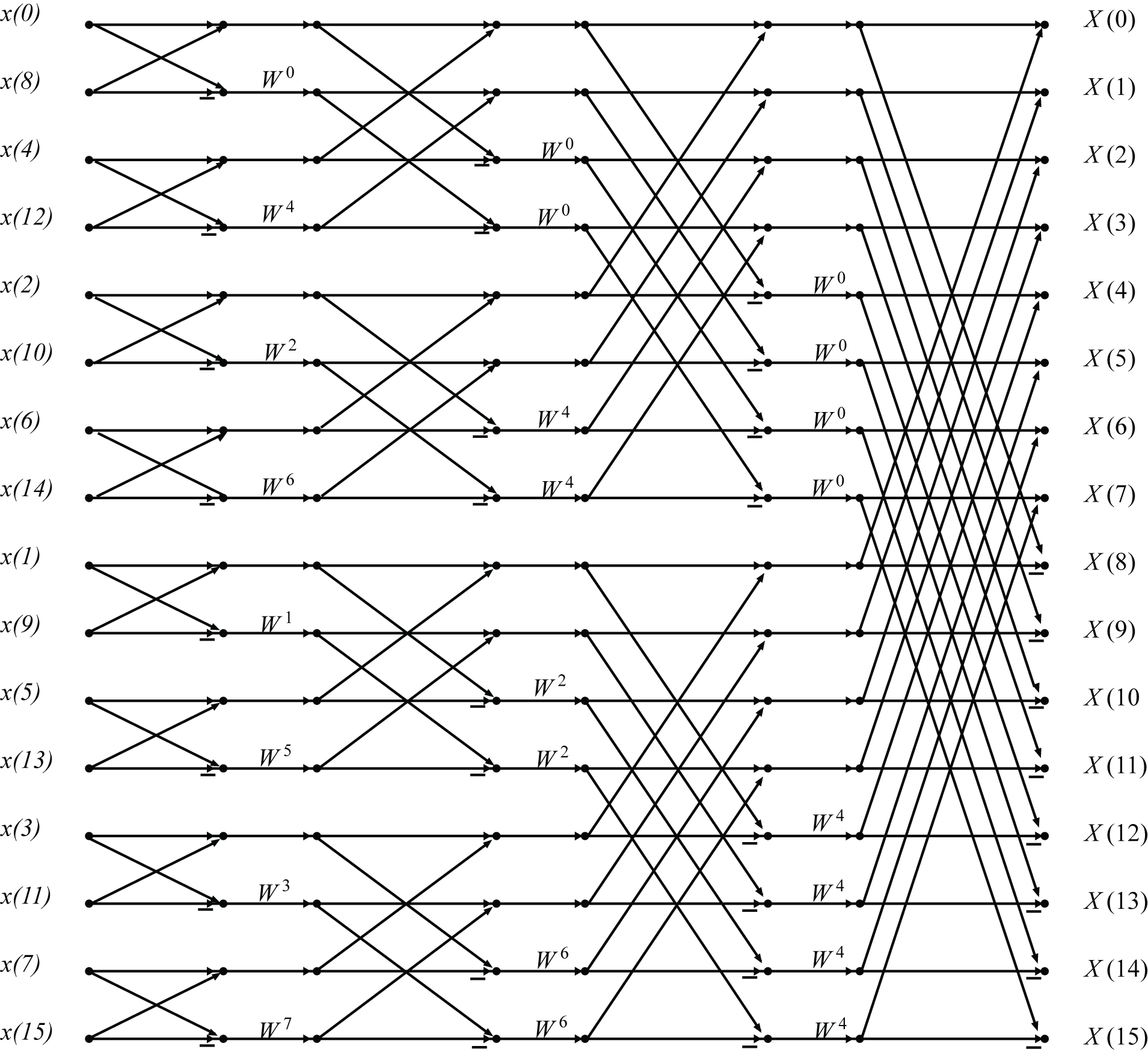
The following four figures are flow graphs for Radix-2 Cooley-Tukey FFTs. The first is a length-16, decimation-in-frequency Radix-2 FFT with the input data in order and output data scrambled. The first stage has 8 length-2 "butterflies" (which overlap in the figure) followed by 8 multiplications by powers of W which are called "twiddle factors". The second stage has 2 length-8 FFTs which are each calculated by 4 butterflies followed by 4 multiplies. The third stage has 4 length-4 FFTs, each calculated by 2 butterflies followed by 2 multiplies and the last stage is simply 8 butterflies followed by trivial multiplies by one. This flow graph should be compared with the index map in Polynomial Description of Signals, the polynomial decomposition in The DFT as Convolution or Filtering, and the program in Appendix 3. In the program, the butterflies and twiddle factor multiplications are done together in the inner most loop. The outer most loop indexes through the stages. If the length of the FFT is a power of two, the number of stages is that power (log N).
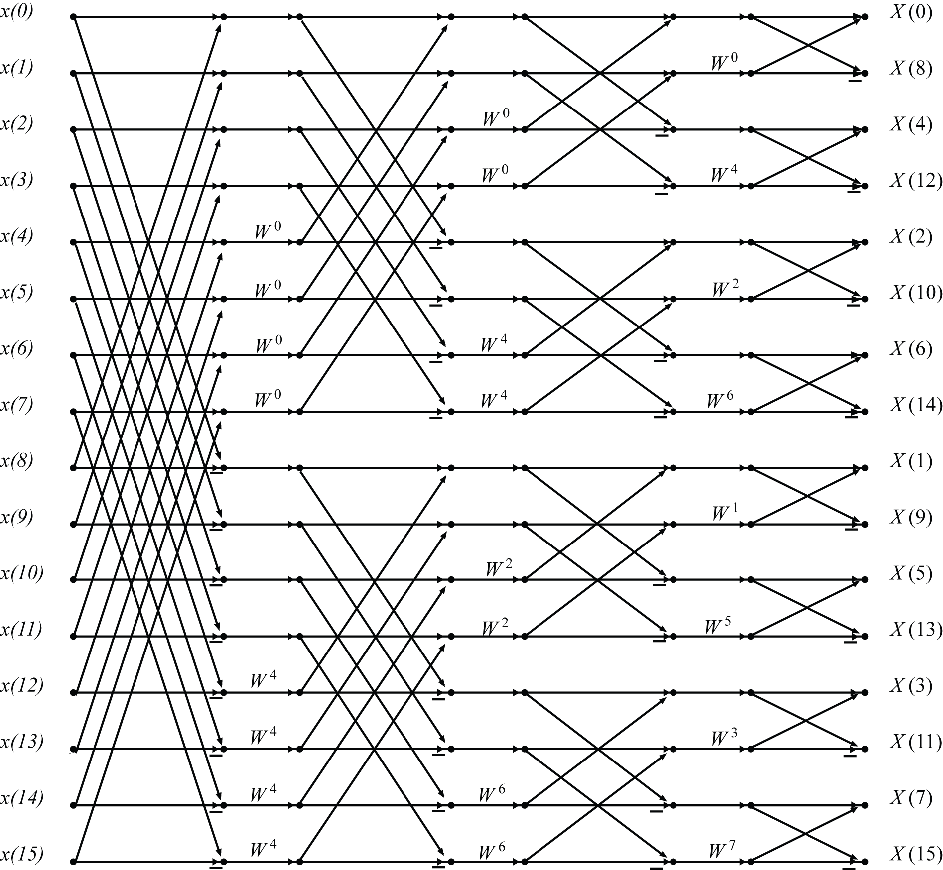
The second figure below is a length-16, decimation-in-time FFT with the input data scrambled and output data in order. The first stage has 8 length-2 "butterflies" followed by 8 twiddle factors multiplications. The second stage has 4 length-4 FFTs which are each calculated by 2 butterflies followed by 2 multiplies. The third stage has 2 length-8 FFTs, each calculated by 4 butterflies followed by 8 multiplies and the last stage is simply 8 length-2 butterflies. This flow graph should be compared with the index map in Polynomial Description of Signals, the polynomial decomposition in The DFT as Convolution or Filtering, and the program in Appendix 3. Here, the FFT must be preceded by a scrambler.
The third and fourth figures below are a length-16 decimation-in-frequency and a decimation-in-time but, in contrast to the figures above, the DIF has the output in order which requires a scrambled input and the DIT has the input in order which requires the output be unscrambled. Compare with the first two figures. Note the order of the twiddle factors. The number of additions and multiplications in all four flow graphs is the same and the structure of the three-loop program which executes the flow graph is the same.


The following is a length-16, decimation-in-frequency Radix-4 FFT with the input data in order and output data scrambled. There are two stages with the first stage having 4 length-4 "butterflies" followed by 12 multiplications by powers of W which are called "twiddle factors. The second stage has 4 length-4 FFTs which are each calculated by 4 butterflies followed by 4 multiplies. Note, each stage here looks like two stages but it is one and there is only one place where twiddle factor multiplications appear. This flow graph should be compared with the index map in Polynomial Description of Signals, the polynomial decomposition in The DFT as Convolution or Filtering, and the program in Appendix 3. Log to the base 4 of 16 is 2. The total number of twiddle factor multiplication here is 12 compared to 24 for the radix-2. The unscrambler is a base-four reverse order counter rather than a bit reverse counter, however, a modification of the radix four butterflies will allow a bit reverse counter to be used with the radix-4 FFT as with the radix-2.

The following two flowgraphs are length-16, decimation-in-frequency Split Radix FFTs with the input data in order and output data scrambled. Because the "butterflies" are L shaped, the stages do not progress uniformly like the Radix-2 or 4. These two figures are the same with the first drawn in a way to compare with the Radix-2 and 4, and the second to illustrate the L shaped butterflies. These flow graphs should be compared with the index map in Polynomial Description of Signals and the program in Appendix 3. Because of the non-uniform stages, the program indexing is more complicated. Although the number of twiddle factor multiplications is 12 as was the radix-4 case, for longer lengths, the split-radix has slightly fewer multiplications than the radix-4.
Because the structures of the radix-2, radix-4, and split-radix FFTs are the same, the number of data additions is same for all of them. However, each complex twiddle factor multiplication requires two real additions (and four real multiplications) the number of additions will be fewer for the structures with fewer multiplications.

