A powerful approach to the development of efficient algorithms is to break a large problem into multiple small ones. One method for doing this with both the DFT and convolution uses a linear change of index variables to map the original one-dimensional problem into a multi-dimensional problem. This approach provides a unified derivation of the Cooley-Tukey FFT, the prime factor algorithm (PFA) FFT, and the Winograd Fourier transform algorithm (WFTA) FFT. It can also be applied directly to convolution to break it down into multiple short convolutions that can be executed faster than a direct implementation. It is often easy to translate an algorithm using index mapping into an efficient program.
The basic definition of the discrete Fourier transform (DFT) is

where n, k, and N are integers,  , the basis functions are the N roots of unity,
and k=0,1,2,⋯,N–1.
If the N values of the transform are calculated from the N values of the data, x(n), it is easily seen that N2 complex multiplications and approximately that same number of complex additions are required. One method for reducing this required arithmetic is to use an index mapping (a change of variables) to change the one-dimensional DFT into a two- or higher dimensional DFT. This is one of the ideas behind the very efficient Cooley-Tukey 6 and Winograd 19 algorithms. The purpose of index mapping is to change a large problem into several easier ones 5, 7. This is sometimes called the “divide and conquer" approach 3 but a more accurate description would be “organize and share" which explains the process of redundancy removal or reduction.
For a length-N sequence, the time index takes on the values
When the length of the DFT is not prime, N can be factored as N=N1N2 and two new independent variables can be defined over the ranges
A linear change of variables is defined which maps n1 and n2 to n and is expressed by

where Ki are integers and the notation ((x))N denotes the integer residue of x modulo N13. This map defines a relation between all possible combinations of n1 and n2 in Equation 3.4 and Equation 3.5 and the values for n in Equation 3.3. The question as to whether all of the n in Equation 3.3 are represented, i.e., whether the map is one-to-one (unique), has been answered in 5 showing that certain integer Ki always exist such that the map in Equation 3.6 is one-to-one. Two cases must be considered.
N1 and N2 are relatively prime, i.e., the greatest common divisor  .
.
The integer map of Equation 3.6 is one-to-one if and only if:

where a and b are integers.
N1 and N2 are not relatively prime, i.e.,  .
.
The integer map of Equation 3.6 is one-to-one if and only if:

or

Reference 5 should be consulted for the details of these conditions and examples. Two classes of index maps are defined from these conditions.
The map of Equation 3.6 is called a type-one map when integers a and b exist such that

The map of Equation 3.6 is called a type-two map when when integers a and b exist such that

The type-one can be used only if the factors of N are relatively prime,
but the type-two can be used whether they are relatively prime or
not. Good 8, Thomas, and Winograd 19 all used the
type-one map in their DFT algorithms. Cooley and Tukey 6
used the type-two in their algorithms, both for a fixed radix  and a mixed radix 17.
The frequency index is defined by a map similar to Equation 3.6 as

where the same conditions, Equation 3.7 and Equation 3.8, are used for determining the uniqueness of this map in terms of the integers K3 and K4.
Two-dimensional arrays for the input data and its DFT are defined using these index maps to give


In some of the following equations, the residue reduction notation will be omitted for clarity. These changes of variables applied to the definition of the DFT given in Equation 3.1 give

where all of the exponents are evaluated modulo N.
The amount of arithmetic required to calculate Equation 3.15 is the same as in the direct calculation of Equation 3.1. However, because of the special nature of the DFT, the integer constants Ki can be chosen in such a way that the calculations are “uncoupled" and the arithmetic is reduced. The requirements for this are

When this condition and those for uniqueness in Equation 3.6 are applied, it is found that the Ki may always be chosen such that one of the terms in Equation 3.16 is zero. If the Ni are relatively prime, it is always possible to make both terms zero. If the Ni are not relatively prime, only one of the terms can be set to zero. When they are relatively prime, there is a choice, it is possible to either set one or both to zero. This in turn causes one or both of the center two W terms in Equation 3.15 to become unity.
An example of the Cooley-Tukey radix-4 FFT for a length-16 DFT uses the type-two map with K1=4, K2=1, K3=1, K4=4 giving
The residue reduction in Equation 3.6 is not needed here since n does not exceed N as n1 and n2 take on their values. Since, in this example, the factors of N have a common factor, only one of the conditions in Equation 3.16 can hold and, therefore, Equation 3.15 becomes

Note the definition of WN in Equation 3.3 allows the simple form of

This has the form of a two-dimensional DFT with an extra
term W16, called a “twiddle factor". The inner
sum over n1 represents four length-4 DFTs, the W16 term
represents 16 complex multiplications, and the outer sum over
n2 represents another four length-4 DFTs. This choice of the
Ki “uncouples" the calculations since the first sum over n1
for n2=0 calculates the DFT of the first row of the data array
 , and those data values are never needed in the
succeeding row calculations. The row calculations are independent,
and examination of the outer sum shows that the column
calculations are likewise independent. This is illustrated in Figure 3.1.
, and those data values are never needed in the
succeeding row calculations. The row calculations are independent,
and examination of the outer sum shows that the column
calculations are likewise independent. This is illustrated in Figure 3.1.
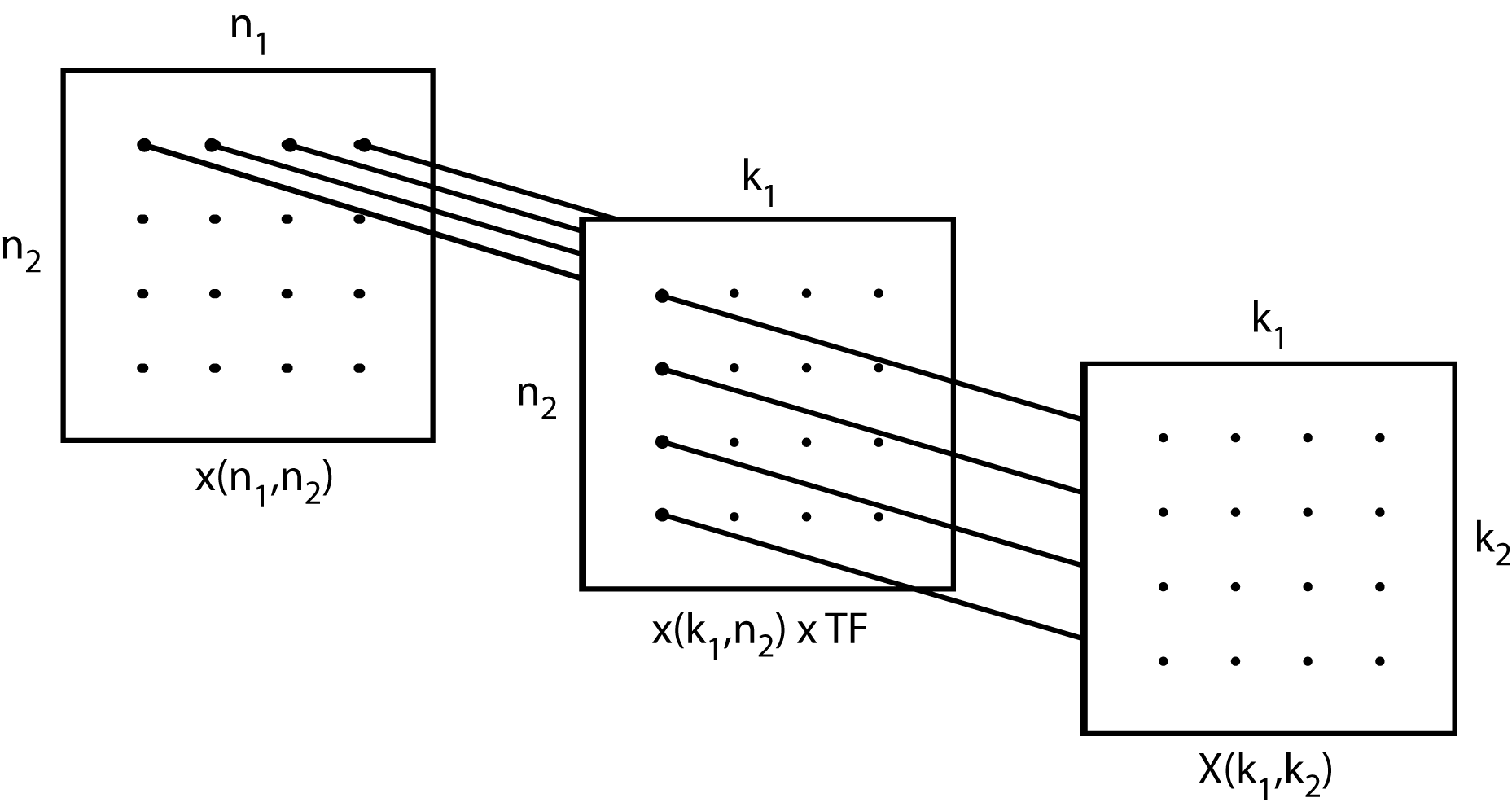
The left 4-by-4 array is the mapped input data, the center array has the rows transformed, and the right array is the DFT array. The row DFTs and the column DFTs are independent of each other. The twiddle factors (TF) which are the center W in Equation 3.19, are the multiplications which take place on the center array of Figure 3.1.
This uncoupling feature reduces the amount of arithmetic required and allows the results of each row DFT to be written back over the input data locations, since that input row will not be needed again. This is called “in-place" calculation and it results in a large memory requirement savings.
An example of the type-two map used when the factors of N are relatively prime is given for N=15 as
The residue reduction is again not explicitly needed. Although the factors 3 and 5 are relatively prime, use of the type-two map sets only one of the terms in Equation 3.16 to zero. The DFT in Equation 3.15 becomes

which has the same form as Equation 3.19, including the existence of the twiddle factors (TF). Here the inner sum is five length-3 DFTs, one for each value of k1. This is illustrated in Equation 3.2 where the rectangles are the 5 by 3 data arrays and the system is called a ``mixed radix" FFT.
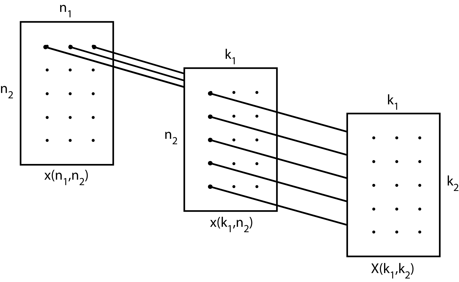
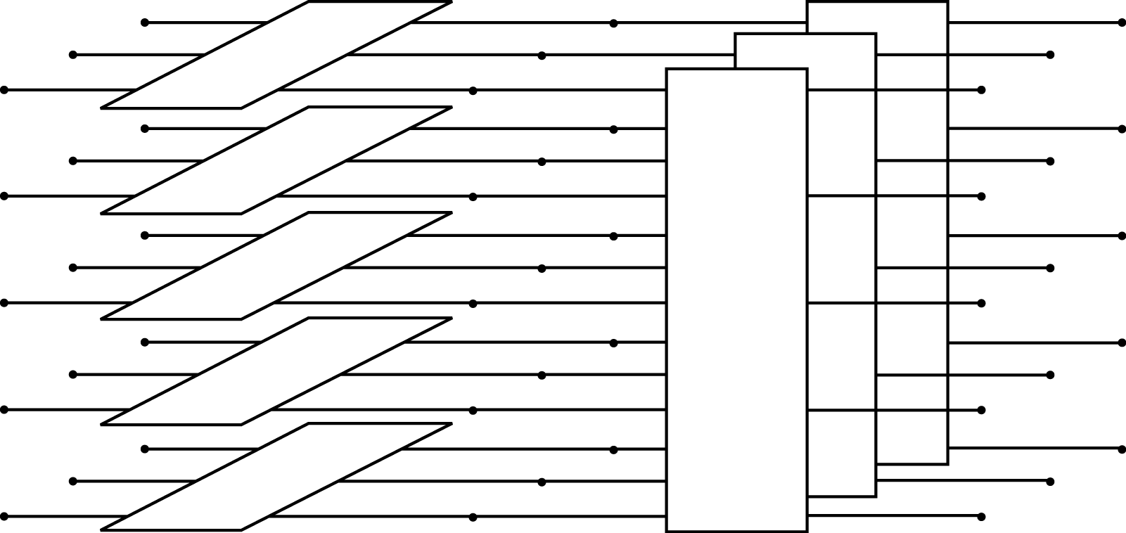
An alternate illustration is shown in Figure 3.3 where the rectangles are the short length 3 and 5 DFTs.
The type-one map is illustrated next on the same length-15 example. This time the situation of Equation 3.7 with the “and" condition is used in Equation 3.10 using an index map of
and
The residue reduction is now necessary. Since the factors of N are relatively prime and the type-one map is being used, both terms in Equation 3.16 are zero, and Equation 3.15 becomes

which is similar to Equation 3.22, except that now the type-one map gives a pure two-dimensional DFT calculation with no TFs, and the sums can be done in either order. Figures Figure 3.2 and Figure 3.3 also describe this case but now there are no Twiddle Factor multiplications in the center and the resulting system is called a ``prime factor algorithm" (PFA).
The purpose of index mapping is to improve the arithmetic efficiency. For example a direct calculation of a length-16 DFT requires 16^2 or 256 real multiplications (recall, one complex multiplication requires 4 real multiplications and 2 real additions) and an uncoupled version requires 144. A direct calculation of a length-15 DFT requires 225 multiplications but with a type-two map only 135 and with a type-one map, 120. Recall one complex multiplication requires four real multiplications and two real additions.
Algorithms of practical interest use short DFT's that require fewer than N2 multiplications. For example, length-4 DFTs require no multiplications and, therefore, for the length-16 DFT, only the TFs must be calculated. That calculation uses 16 multiplications, many fewer than the 256 or 144 required for the direct or uncoupled calculation.
The concept of using an index map can also be applied to
convolution to convert a length N=