Acknowledgment: This appendix, written with assistance from Cédric J. Demeure and Peter Massey, was inspired by the MATLAB user's manual from The MATHWORKS, Inc. The MA TLAB Primer, available through the MATLAB User's Group, is a useful learning aid for teachers and students. To join the MATLAB User's Group, send your request via E-mail to matlab-users request@mcs.anl.gov.

In order to run MATLAB on a Macintosh SE or PLUS computer, you need the program called EDU-MATLAB. The program requires at least 1 Mbyte of memory, System 3.0 or above, Finder version 3.0 or above, and an 800K drive. A hard disc drive is highly recommended. In order to run MATLAB on a Macintosh II, IIx, IIcx, or SE/30, you need the program called MacII-MATLAB, and the same system requirements apply.

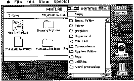
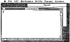
To start MATLAB, you may need to open the folder containing the MATLAB program. Then just “double-click” the program icon or the program name (for example, EDU-MATLAB). Figure A.1 shows a typical organization of the folder containing Mac II-MATLAB. It contains the main program, the settings file, the demonstrations folder, and any toolbox folders. The double-click on Mac II-MATLAB produces the Command window as shown in Figure A.2. You will also see a Graph window partially hidden behind it. (The fact that the window is not in ffont means that it is opened but not currently active.) If you do not know what “clicking,” “dragging,” “pop-up menu,” and “trash” mean, you should stop reading now and familiarize yourself with the Macintosh.

Figure 8.1. 

The MATLAB Folder (©Apple Computer, Inc., used with permission.)

In the command window, you should see the prompt ≫. The program interpreter is waiting for you to enter instructions. At this point it is a good idea to run the demonstration programs that are available in the “About MATLAB” menu under the Apple menu. Just click on the “demos” button and select a demo. During pauses, strike any key to continue. Whenever you have a MATLAB file in any folder, then you may double-click the file to launch the program. This allows you to have your own folder containing your own MATLAB files, separated from the MATLAB folder.

Figure 8.2. 

The Command Window (©Apple Computer, Inc., used with permission.)

MATLAB has four types of windows:

All windows follow the traditional behavior of Macintosh windows. You can resize them (actually the help window has a fixed size) or move them. For more details on menus and windows, see the Macintosh and MATLAB manuals.

In order to run MATLAB (Version 3.5) on an IBM or compatible personal computer, you must have a floating point math coprocessor (80x87)installed and at least 512 kbytes of memory. The program is called PCMAT-LAB.EXE, but it is usually invoked via the batch file MATLAB.BAT in the MATLAB subdirectory. If you are using a menu system and MATLAB is one of your choices, just choose it. Otherwise, go to the MATLAB suiUirectory and type MATLAB.

You may be able to usea more powerful implementation of MATLAB if you have an 80286 or 80386 machine. AT-MATLAB runs on an 80286 with at least 1 Mbyte of extended memory. AT-MATLAB is distributed with PC-MATLAB. 386-MATLAB, a special version for 80386 or 80486 machines with virtual memory support and no limits on variable size, is sold separately.

When you run MATLAB, you should see the prompt ≫. The program interpreter is waiting for you to enter instructions. Some MATLAB instructions, such as plot, are graphics-type instructions which plot results and data. Execution of one of these graphics instructions puts the PC screen into the graphics mode, which displays the resulting plot. No instructions can be executed in the graphics mode other than a screen-dump function. Striking any other key will return the PC to the command mode, but the graphics are temporarily stored (like variables) and can be recalled by the shg (show graphics) instruction. If you wish, you may run some of the demonstration programs now by entering demo and following the on-screen instructions.

In command mode, MATLAB displays a prompt (≫) and waits for your input. You may type any legal mathematical expression for immediate evaluation. Try the following three examples (press “enter” or “return” at the end of each line):

≫ 2+2
≫ 5^2
≫ 2*sin(pi/4)

The variable pi = 3.14 is built into MATLAB, as are the sin function and hundreds of other functions. When you entered each of the preceding lines, MATLAB stored the results in a variable called ans for answer. The value of ans was then displayed. The last line should have produced the square root of 2. We can manipulate ans to find out

≫ ans^2

The new answer is very close to 2, as expected. Let's see what the roundoff error is:

≫ ans-2

Any result you wish to keep for a while may be assigned to a variable other than ans:

≫ x = pi/7
≫ cos(x)
≫ y = sin(x)^2+cos(x)^2;
≫ y

A semicolon (;) at the end of the line suppresses printing of the result, as when we calculated y in the next-to-last line just shown. This feature is especially useful when writing MATLAB programs where intermediate results are not of interest and when working with large matrices.

MATLAB supports the dynamic creation of variables. You can create your own variables by just assigning a value to a variable. For example, type x = 3.5+4.2. Then the real variable x contains the value 7.7. Variable names must start with an alphabetical character and be less than nineteen characters long. If you type x = -3*4.0, the content 7.7 is replaced by the value -12. Some commands allow you to keep track of all the variables that you have already created in your session. Type who or whos to get the list and names of the variables currently in memory (whos gives more information than who). To clear all the variables, type in clear. To clear a single variable (or several) from the list, follow the command clear by the name of the variable you want to delete or by a list of variable names separated by spaces. Try it now.

MATLAB is case sensitive. In other words, x and X are two different variables. You can control the case sensitivity of MATLAB by entering the command casesen, which toggles the sensitivity. The command casesen on enforces case sensitivity, and casesen off cancels it.

If one line is not enough to enter your command, then finish the first line with two dots (. . ) and continue on the next line. You can enter more than one command per line by separating them with commas if you want the result displayed or with semicolons if you do not want the result displayed. For example, type

≫ theta = pi/7; x = cos(theta); y = sin(theta);
≫ x,y

to first compute theta,cos(theta), and sin(theta) and then to print x and y .

The number is predefined in MATLAB and stored in the two variable locations denoted by i and j. This double definition comes from the preference of mathematicians for using i and the preference of engineers for using j (with i denoting electrical current). i and j are variables, and their contents may be changed. If you type j = 5, then this is the value for j and j no longer contains . Type in j = sqrt(-1) to restore the original value. Note the way a complex variable is displayed. If you type i, you should get the answer

i =
    0+1.0000i.

The same value will be displayed for j. Try it. Using j, you can now enter complex variables. For example, enter z1 = 1+2*j and z2 = 2+1.5*j. As j is a variable, you have to use the multiplication sign *. Otherwise, you will get an error message. MATLAB does not differentiate (except in storage) between a real and a complex variable. Therefore variables may be added, subtracted, multiplied, or even divided. For example, type in x = 2, z = 4.5*j, and z/x. The real and imaginary parts of z are both divided by x. MATLAB just treats the real variable x as a complex variable with a zero imaginary part. A complex variable that happens to have a zero imaginary part is treated like a real variable. Subtract 2*j from z1 and display the result.

MATLAB contains several built-in functions to manipulate complex numbers. For example, real (z) extracts the real part of the complex number z. Type

≫ z = 2+1.5*j, real(z)

to get the result

z =
   2.000+1.500i

ans =
   2

Similarly, imag(z) extracts the imaginary part of the complex number z. The functions abs(z) and angle(z) compute the absolute value (magnitude) of the complex number z and its angle (in radians). For example, type

≫ z = 2+2*j;
≫ r = abs(z)
≫ theta = angle(z)
≫ z = r*exp(j*theta)

The last command shows how to get back the original complex number from its magnitude and angle. This is clarified in Chapter 1: Complex Numbers.

Another useful function, conj (z), returns the complex conjugate of the complex number z. If z = x+j*y where x and y are real, then conj (z) is equal to x-j*y. Verify this for several complex numbers by using the function conj (z).

As its name indicates, MATLAB is especially designed to handle matrices. The simplest way to enter a matrix is to use an explicit list. In the list, the elements are separated by blanks or commas, and the semicolon (;) is used to indicate the end of a row. The list is surrounded by square brackets . For example, the statement

≫ A = [1 2 3;4 5 6;7 8 9]

results in the output

A = 
   1 2 3
   4 5 6
   7 8 9

The variable A is a matrix of size 3×3. Matrix elements can be any MATLAB expression. For example, the command

≫ x = [-1.3 sqrt(3) (1+2+3)*4/5]

results in the matrix

x = 
   -1.3000  1.7321  4.8000

We call a matrix with just one row or one column a vector, and a 1×1 matrix is a scalar. Individual matrix elements can be referenced with indices that are placed inside parentheses. Type x(5) = abs(x(1)) to produce the new vector

x = 
   -1.3000  1.7321  4.8000  0.000  1.3000

Note that the size of x has been automatically adjusted to accommodate the new element and that elements not referenced are set equal to 0 (here x(4)). New rows or columns can be added very easily. Try typing r = [10 11 12],A = [A;r]. Dimensions in the command must coincide. Try r = [13 14],A = [A;r].

The command size(A) gives the number of rows and the number of columns of A. The output from size(A) is itself a matrix of size 1×2. These numbers can be stored if necessary by the command [m n] = size(A). In our previous example, A = [A;r] is a 4×3 matrix, so the variable m will contain the number 4 and n will contain the number 3. A vector is a matrix for which either m or n is equal to 1. If m is equal to 1, the matrix is a row vector; if n is equal to 1, the matrix is a column vector. Matrices and vectors may contain complex numbers. For example, the statement

≫ A = [1 2;3 4]+j*[5 6;7 8]

and the statement

≫ A = [1+5*j 2+6*j;3+7*j 4+8*j]

are equivalent, and they both produce the matrix

A =
   1.0000+5.0000i    2.0000+6.0000i
   3.0000+7.0000i    4.0000+8.0000i

Note that blanks must be avoided in the second expression for A. Try typing

≫A = [1 + 5*j 2 + 6*j 2 + 6*j;3 +7*j 4 + 8*j]

What is the size of A now?

MATLAB has several built-in functions to manipulate matrices. The special character, ', for prime denotes the transpose of a matrix. The statement A = [ 1 2 3;4 5 6;7 8 9]' produces the matrix

A = 
   1 4 7 
   2 5 8
   3 6 9

The rows of A' are the column of A, and vice versa. If A is a complex matrix, then A is its complex conjugate transpose or hermitian transpose. For an “unconjugate” transpose, use the two-character operator dot-prime (. '). Matrix and vector variables can be added, subtracted, and multiplied as regular variables if the sizes match. Only matrices of the same size can be added or subtracted. There is, however, an easy way to add or subtract a common scalar from each element of a matrix. For example, x = [1 2 3 4],x = x-1 produces the output

x = 
   1 2 3 4

x = 
   0 1 2 3

As discussed in the chapter on linear algebra, multiplication of two matrices is only valid if the inner sizes of the matrices are equal. In other words, A*B is valid if the second size of A (number of columns) is the same as the first size of B (number of rows). Let a_i,j represent the element of A in the i^th row and the j^th column. Then the matrix A*B consists of elements

(8.1)

where n is the number of columns of A and the number of rows of B. Try typing A = [1 2 3;4 5 6];B = [7;8;9]; A*B. You should get the result

ans =
    50
    112

The inner product between two column vectors x and y is the scalar defined as the product x'*y or equivalently as y'*x For example, x = [1;2],y = [3;4],x'*y, leads to the result

ans =
    11

Similarly, for row vectors the inner product is defined as x*y'. The Euclidean norm of a vector is defined as the square root of the inner product between a vector and itself. Try to compute the norm of the vector [1 2 3 4]. You should get 5.4772. The outer product of two column (row) vectors is the matrix x*y' (x'*y).

Any scalar can multiply or be multiplied by a matrix. The multiplication is then performed element by element. Try A = [1 2 3;4 5 6;7 8 9];A*2. You should get

ans =
    2  4  6
    8 10 12
   14 26 28

Verify that 2*A gives the same result.

The inverse of a matrix is computed by using the function inv(A) and is only valid if A is square. If the matrix is singular, meaning that it has no inverse, a message will appear. Try typing inv(A). You should get

Warning: Matrix is close to singular or badly scaled.
   Results may be inaccurate. RCOND=2.937385e-18

ans =
     1.0e+16*
     0.3152  -0.6304   0.3152
    -0.6304   1.2609  -0.6304
     0.3152  -0.6304   0.3152  

The inverse of a matrix may be used to solve a linear system of equations. For example, to solve the system

you could type A = [1 2 3;1 -2 4;0 -2 1]; b = [2;7;3]; inv(A)*b and get

ans =
    1
   -1
    1

(8.2)

Check to see that this is the correct answer by typing A*[1;-1;1]. What do you see?

MATLAB offers another way to solve linear systems, based on Gauss elimination, that is faster than computing the inverse. The syntax is A\b and is valid whenever A has the same number of rows as b. Try it.

The “Dot” Operator. Sometimes you may want to perform an operation element by element. In MATLAB, these element-by-element operations are called array operations. Of course, matrix addition and subtraction are already element-by-element operations. The operation A. *B denotes the multiplication, element by element, of the matrices A and B. Make two 3 ×3 matrices, A and B, and try

≫ A*B
≫ A.*B

Suppose we want to find the square of each number in A. The proper way to specify this calculation is

≫ A_squared=A.^2

where the period (dot)