Now imagine that we create an account with $10 in it. Let us think about what happens if we withdraw too
much money from the account. If we do these transactions in order, we receive an insufficient funds message.
>>> w = make_withdraw(10)
>>> w(8)
2
>>> w(7)
’Insufficient funds’
In parallel, however, there can be many different outcomes. One possibility appears below:
P1: w(8)
P2: w(7)
read balance: 10
read amount: 8
read balance: 10
8 > 10: False
read amount: 7
if False
7 > 10: False
10 - 8: 2
if False
6
write balance -> 2
10 - 7: 3
read balance: 2
write balance -> 3
print 2
read balance: 3
print 3
This particular example gives an incorrect outcome of 3. It is as if the w(8) transaction never happened!
Other possible outcomes are 2, and ’Insufficient funds’. The source of the problems are the following:
if P2 reads balance before P1 has written to balance (or vice versa), P2’s state is inconsistent. The value of
balance that P2 has read is obsolete, and P1 is going to change it. P2 doesn’t know that and will overwrite it
with an inconsistent value.
These example shows that parallelizing code is not as easy as dividing up the lines between multiple processors
and having them be executed. The order in which variables are read and written matters.
A tempting way to enforce correctness is to stipulate that no two programs that modify shared data can run at
the same time. For banking, unfortunately, this would mean that only one transaction could proceed at a time, since
all transactions modify shared data. Intuitively, we understand that there should be no problem allowing 2 different
people to perform transactions on completely separate accounts simultaneously. Somehow, those two operations
do not interfere with each other the same way that simultaneous operations on the same account interfere with
each other. Moreover, there is no harm in letting processes run concurrently when they are not reading or writing.
4.3.2 Correctness in Parallel Computation
There are two criteria for correctness in parallel computation environments. The first is that the outcome should
always be the same. The second is that the outcome should be the same as if the code was executed in serial.
The first condition says that we must avoid the variability shown in the previous section, in which interleaving
the reads and writes in different ways produces different results. In the example in which we withdrew w(8) and
w(7) from a $10 account, this condition says that we must always return the same answer independent of the
order in which P1’s and P2’s instructions are executed. Somehow, we must write our programs in such a way
that, no matter how they are interleaved with each other, they should always produce the same result.
The second condition pins down which of the many possible outcomes is correct. In the example in which
we evaluated w(7) and w(8) from a $10 account, this condition says that the result must always come out to be
Insufficient funds, and not 2 or 3.
Problems arise in parallel computation when one process influences another during critical sections of a pro-
gram. These are sections of code that need to be executed as if they were a single instruction, but are actually
made up of smaller statements. A program’s execution is conducted as a series of atomic hardware instructions,
which are instructions that cannot be broken in to smaller units or interrupted because of the design of the proces-
sor. In order to behave correctly in concurrent situations, the critical sections in a programs code need to be have
atomicity -- a guarantee that they will not be interrupted by any other code.
To enforce the atomicity of critical sections in a program’s code under concurrency , there need to be ways to
force processes to either serialize or synchronize with each other at important times. Serialization means that only
one process runs at a time -- that they temporarily act as if they were being executed in serial. Synchronization
takes two forms. The first is mutual exclusion, processes taking turns to access a variable, and the second is
conditional synchronization, processes waiting until a condition is satisfied (such as other processes having
finished their task) before continuing. This way, when one program is about to enter a critical section, the other
processes can wait until it finishes, and then proceed safely.
4.3.3 Protecting Shared State: Locks and Semaphores
All the methods for synchronization and serialization that we will discuss in this section use the same underlying
idea. They use variables in shared state as signals that all the processes understand and respect. This is the same
philosophy that allows computers in a distributed system to work together -- they coordinate with each other by
passing messages according to a protocol that every participant understands and respects.
These mechanisms are not physical barriers that come down to protect shared state. Instead they are based on
mutual understanding. It is the same sort of mutual understanding that allows traffic going in multiple directions to
safely use an intersection. There are no physical walls that stop cars from crashing into each other, just respect for
rules that say red means “stop”, and green means “go”. Similarly, there is really nothing protecting those shared
7
variables except that the processes are programmed only to access them when a particular signal indicates that it
is their turn.
Locks. Locks, also known as mutexes (short for mutual exclusions), are shared objects that are commonly
used to signal that shared state is being read or modified. Different programming languages implement locks in
different ways, but in Python, a process can try to acquire “ownership” of a lock using the acquire() method,
and then release() it some time later when it is done using the shared variables. While a lock is acquired by
a process, any other process that tries to perform the acquire() action will automatically be made to wait until
the lock becomes free. This way, only one process can acquire a lock at a time.
For a lock to protect a particular set of variables, all the processes need to be programmed to follow a rule: no
process will access any of the shared variables unless it owns that particular lock. In effect, all the processes need
to “wrap” their manipulation of the shared variables in acquire() and release() statements for that lock.
We can apply this concept to the bank balance example. The critical section in that example was the set of
operations starting when balance was read to when balance was written. We saw that problems occurred if
more than one process was in this section at the same time. To protect the critical section, we will use a lock.
We will call this lock balance_lock (although we could call it anything we liked). In order for the lock to
actually protect the section, we must make sure to acquire() the lock before trying to entering the section, and
release() the lock afterwards, so that others can have their turn.
>>> from threading import Lock
>>> def make_withdraw(balance):
balance_lock = Lock()
def withdraw(amount):
nonlocal balance
# try to acquire the lock
balance_lock.acquire()
# once successful, enter the critical section
if amount > balance:
print("Insufficient funds")
else:
balance = balance - amount
print(balance)
# upon exiting the critical section, release the lock
balance_lock.release()
If we set up the same situation as before:
w = make_withdraw(10)
And now execute w(8) and w(7) in parallel:
P1
P2
acquire balance_lock: ok
read balance: 10
acquire balance_lock: wait
read amount: 8
wait
8 > 10: False
wait
if False
wait
10 - 8: 2
wait
write balance -> 2
wait
read balance: 2
wait
print 2
wait
release balance_lock
wait
acquire balance_lock:ok
read balance: 2
read amount: 7
7 > 2: True
if True
print ’Insufficient funds’
release balance_lock
8
We see that it is impossible for two processes to be in the critical section at the same time. The instant one
process acquires balance_lock, the other one has to wait until that processes finishes its critical section before it
can even start.
Note that the program will not terminate unless P1 releases balance_lock. If it does not release balance_lock,
P2 will never be able to acquire it and will be stuck waiting forever. Forgetting to release acquired locks is a com-
mon error in parallel programming.
Semaphores. Semaphores are signals used to protect access to limited resources. They are similar to locks,
except that they can be acquired multiple times up to a limit. They are like elevators that can only carry a certain
number of people. Once the limit has been reached, a process must wait to use the resource until another process
releases the semaphore and it can acquire it.
For example, suppose there are many processes that need to read data from a central database server. The
server may crash if too many processes access it at once, so it is a good idea to limit the number of connections.
If the database can only support N=2 connections at once, we can set up a semaphore with value N=2.
>>> from threading import Semaphore
>>> db_semaphore = Semaphore(2) # set up the semaphore
>>> database = []
>>> def insert(data):
db_semaphore.acquire() # try to acquire the semaphore
database.append(data)
# if successful, proceed
db_semaphore.release() # release the semaphore
>>> insert(7)
>>> insert(8)
>>> insert(9)
The semaphore will work as intended if all the processes are programmed to only access the database if they
can acquire the semaphore. Once N=2 processes have acquired the semaphore, any other processes will wait until
one of them has released the semaphore, and then try to acquire it before accessing the database:
P1
P2
P3
acquire db_semaphore: ok
acquire db_semaphore: wait
acquire db_semaphore: ok
read data: 7
wait
read data: 9
append 7 to database
wait
append 9 to database
release db_semaphore: ok
acquire db_semaphore: ok
release db_semaphore: ok
read data: 8
append 8 to database
release db_semaphore: ok
A semaphore with value 1 behaves like a lock.
4.3.4 Staying Synchronized: Condition variables
Condition variables are useful when a parallel computation is composed of a series of steps. A process can use a
condition variable to signal it has finished its particular step. Then, the other processes that were waiting for the
signal can start their work. An example of a computation that needs to proceed in steps a sequence of large-scale
vector computations. In computational biology, web-scale computations, and image processing and graphics, it is
common to have very large (million-element) vectors and matrices. Imagine the following computation:
9
We may choose to parallelize each step by breaking up the matrices and vectors into range of rows, and
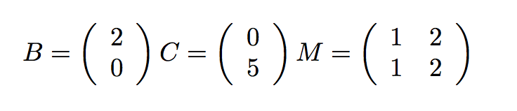
assigning each range to a separate thread. As an example of the above computation, imagine the following simple
values:
We will assign first half (in this case the first row) to one thread, and the second half (second row) to another
thread:
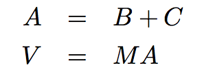
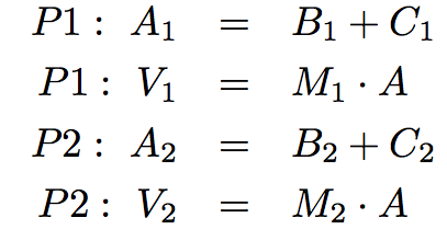
In pseudocode, the computation is:
def do_step_1(index):
A[index] = B[index] + C[index]
def do_step_2(index):
V[index] = M[index] . A
Process 1 does:
do_step_1(1)
do_step_2(1)
And process 2 does:
do_step_1(2)
do_step_2(2)
If allowed to proceed without synchronization, the following inconsistencies could result:
P1
P2
read B1: 2
read C1: 0
calculate 2+0: 2
write 2 -> A1
read B2: 0
read M1: (1 2)
read C2: 5
read A: (2 0)
calculate 5+0: 5
calculate (1 2).(2 0): 2
write 5 -> A2
write 2 -> V1
read M2: (1 2)
read A: (2 5)
calculate (1 2).(2 5):12
write 12 -> V2
10
The problem is that V should not be computed until all the elements of A have been computed. However, P1
finishes A = B+C and moves on to V = MA before all the elements of A have been computed. It therefore uses
an inconsistent value of A when multiplying by M.
We can use a condition variable to solve this problem.
Condition variables are objects that act as signals that a condition has been satisfied. They are commonly
used to coordinate processes that need to wait for something to happen before continuing. Processes that need the
condition to be satisfied can make themselves wait on a condition variable until some other process modifies it to
tell them to proceed.
In Python, any number of processes can signal that they are waiting for a condition using the condition.wait()
method. After calling this method, they automatically wait until some other process calls the condition.notify()
or condition.notifyAll() function. The notify() method wakes up just one process, and leaves the
others waiting. The notifyAll() method wakes up all the waiting processes. Each of these is useful in differ-
ent situations.
Since condition variables are usually associated with shared variables that determine whether or not the con-
dition is true, they are offer acquire() and release() methods. These methods should be used when
modifying variables that could change the status of the condition. Any process wishing to signal a change in the
condition must first get access to it using acquire().
In our example, the condition that must be met before advancing to the second step is that both processes must
have finished the first step. We can keep track of the number of processes that have finished a step, and whether
or not the condition has been met, by introducing the following 2 variables:
step1_finished = 0
start_step2 = Condition()
We will insert a start_step_2().wait() at the beginning of do_step_2. Each process will increment
step1_finished when it finishes Step 1, but we will only signal the condition when step_1_finished
= 2. The following pseudocode illustrates this:
step1_finished = 0
start_step2 = Condition()
def do_step_1(index):
A[index] = B[index] + C[index]
# access the shared state that determines the condition status
start_step2.acquire()
step1_finished += 1
if(step1_finished == 2): # if the condition is met
start_step2.notifyAll() # send the signal
#release access to shared state
start_step2.release()
def do_step_2(index):
# wait for the condition
start_step2.wait()
V[index] = M[index] . A
With the introduction of this condition, both processes enter Step 2 together as follows::
P1
P2
read B1: 2
read C1: 0
calculate 2+0: 2
write 2 -> A1
read B2: 0
acquire start_step2: ok
read C2: 5
write 1 -> step1_finished
calculate 5+0: 5
step1_finished == 2: false
write 5-> A2
release start_step2: ok
acquire start_step2: ok
start_step2: wait
write 2-> step1_finished
11
wait
step1_finished == 2: true
wait
notifyAll start_step_2: ok
start_step2: ok
start_step2:ok
read M1: (1 2)
read M2: (1 2)
read A:(2 5)
calculate (1 2). (2 5): 12
read A:(2 5)
write 12->V1
calculate (1 2). (2 5): 12
write 12->V2
Upon entering do_step_2, P1 has to wait on start_step_2 until P2 increments step1_finished,
finds that it equals 2, and signals the condition.
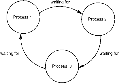
4.3.5 Deadlock
While synchronization methods are effective for protecting shared state, they come with a catch. Because they
cause processes to wait on each other, they are vulnerable to deadlock, a situation in which two or more processes
are stuck, waiting for each other to finish. We have already mentioned how forgetting to release a lock can cause a
process to get stuck indefinitely. But even if there are the correct number of acquire() and release() calls,
programs can still reach deadlock.
The source of deadlock is a circular wait, illustrated below. No process can continue because it is waiting for
other processes that are waiting for it to complete.
As an example, we will set up a deadlock with two processes. Suppose there are two locks, x_lock and
y_lock, and they are used as follows:
>>> x_lock = Lock()
>>> y_lock = Lock()
>>> x = 1
>>> y = 0
>>> def compute():
x_lock.acquire()
y_lock.acquire()
y = x + y
12
x = x * x
y_lock.release()
x_lock.release()
>>> def anti_compute():
y_lock.acquire()
x_lock.acquire()
y = y - x
x = sqrt(x)
x_lock.release()
y_lock.release()
If compute() and anti_compute() are executed in parallel, and happen to interleave with each other as
follows:
P1
P2
acquire x_lock: ok
acquire y_lock: ok
acquire y_lock: wait
acquire x_lock: wait
wait
wait
wait
wait
wait
wait
...
...
the resulting situation is a deadlock. P1 and P2 are each holding on to one lock, but they need both in order
to proceed. P1 is waiting for P2 to release y_lock, and P2 is waiting for P1 to release x_lock. As a result,
neither can proceed.
13
Chapter 5: Sequences and Coroutines
Contents
5.1 Introduction
In this chapter, we continue our discussion of real-world applications by developing new tools to process sequential
data. In Chapter 2, we introduced a sequence interface, implemented in Python by built-in data types such as
tuple and list. Sequences supported two operations: querying their length and accessing an element by
index. In Chapter 3, we developed a user-defined implementations of the sequence interface, the Rlist class for
representing recursive lists. These sequence types proved effective for representing and accessing a wide variety
of sequential datasets.
However, representing sequential data using the sequence abstraction has two important limitations. The first
is that a sequence of length n typically takes up an amount of memory proportional to n. Therefore, the longer a
sequence is, the more memory it takes to represent it.
The second limitation of sequences is that sequences can only represent datasets of known, finite length. Many
sequential collections that we may want to represent do not have a well-defined length, and some are even infinite.
Two mathematical examples of infinite sequences are the positive integers and the Fibonacci numbers. Sequential
data sets of unbounded length also appear in other computational domains. For instance, the sequence of all
Twitter posts grows longer with every second and therefore does not have a fixed length. Likewise, the sequence
of telephone calls sent through a cell tower, the sequence of mouse movements made by a computer user, and the
sequence of acceleration measurements from sensors on an aircraft all extend without bound as the world evolves.
In this chapter, we introduce new constructs for working with sequential data that are designed to accommodate
collections of unknown or unbounded length, while using limited memory. We also discuss how these tools can
be used with a programming construct called a coroutine to create efficient, modular data processing pipelines.
5.2 Implicit Sequences
The central observation that will lead us to efficient processing of sequential data is that a sequence can be repre-
sented using programming constructs without each element being stored explicitly in the memory of the computer.
To put this idea into practice, we will construct objects that provides access to all of the elements of some sequen-
tial dataset that an application may desire, but without computing all of those elements in advance and storing
them.
A simple example of this idea arises in the range sequence type introduced in Chapter 2. A range represents
a consecutive, bounded sequence of integers. However, it is not the case that each element of that sequence is
represented explicitly in memory. Instead, when an element is requested from a range, it is computed. Hence,
we can represent very large ranges of integers without using large blocks of memory. Only the end points of the
range are stored as part of the range object, and elements are computed on the fly.
>>> r = range(10000, 1000000000)
>>> r[45006230]
45016230
In this example, not all 999,990,000 integers in this range are stored when the range instance is constructed.
Instead, the range object adds the first element 10,000 to the index 45,006,230 to produce the element 45,016,230.
Computing values on demand, rather than retrieving them from an existing representation, is an example of lazy
computation. Computer science is a discipline that celebrates laziness as an important computational tool.
1
An iterator is an object that provides sequential access to an underlying sequential dataset. Iterators are built-
in objects in many programming languages, including Python. The iterator abstraction has two components: a
mechanism for retrieving the next element in some underlying series of elements and a mechanism for signaling
that the end of the series has been reached and no further elements remain. In programming languages with built-in
object systems, this abstraction typically corresponds to a particular interface that can be implemented by classes.
The Python interface for iterators is described in the next section.
The usefulness of iterators is derived from the fact that the underlying series of data for an iterator may not be
represented explicitly in memory. An iterator provides a mechanism for considering each of a series of values in
turn, but all of those elements do not need to be stored simultaneously. Instead, when the next element is requested
from an iterator, that element may be computed on demand instead of being retrieved from an existing memory
source.
Ranges are able to compute the elements of a sequence lazily because the sequence represented is uniform,
and any element is easy to compute from the starting and ending bounds of the range. Iterators allow for lazy
generation of a much broader class of underlying sequential datasets, because they do not need to provide access
to arbitrary elements of the underlying series. Instead, they must only compute the next element of the series,
in order, each time another element is requested. While not as flexible as accessing arbitrary elements of a
sequence (called random access), sequential access to sequential data series is often sufficient for data processing
applications.
5.2.1 Python Iterators
The Python iterator interface includes two messages. The __next__ message queries the iterator for the next
element of the underlying series that it represents. In response to invoking __next__ as a method, an iterator
can perform arbitrary