This chapter is published by NCPEA Press and is presented as an NCPEA/Connexions publication "print on demand book." Each chapter has been peer-reviewed, accepted, and endorsed by the National Council of Professors of Educational Administration (NCPEA) as a significant contribution to the scholarship and practice of education administration.
| John R. Slate is a Professor at Sam Houston State University where he teaches Basic and Advanced Statistics courses, as well as professional writing, to doctoral students in Educational Leadership and Counseling. His research interests lie in the use of educational databases, both state and national, to reform school practices. To date, he has chaired and/or served over 100 doctoral student dissertation committees. Recently, Dr. Slate created a website (Writing and Statistical Help) to assist students and faculty with both statistical assistance and in editing/writing their dissertations/theses and manuscripts. |
| Ana Rojas-LeBouef is a Literacy Specialist at the Reading Center at Sam Houston State University where she teaches developmental reading courses. Dr. LeBoeuf recently completed her doctoral degree in Reading, where she conducted a 16-year analysis of Texas statewide data regarding the achievement gap. Her research interests lie in examining the inequities in achievement among ethnic groups. Dr. Rojas-LeBouef also assists students and faculty in their writing and statistical needs on the Writing and Statistical Help website.
|
In this set of steps, readers will calculate a multivariate analysis of variance procedure, following the determination of the extent to which data for the dependent variables reflect normal distributions. Although a parametric statistical procedure requires that its data be reflective of a normal curve, the multivariate analysis of variance procedure is regarded as being sufficiently robust that it can withstand most violations. For detailed information regarding the assumptions underlying the multivariate analysis of variance (MANOVA) procedure, readers are referred to the Hyperstats Online Statistics Textbook at http://davidmlane.com/hyperstat/ ; to the Electronic Statistics Textbook (2011) at http://www.statsoft.com/textbook/ ; or to Andy Field’s (2009) Discovering Statistics Using SPSS at http://www.amazon.com/Discovering-Statistics-Introducing-Statistical-Method/dp/1847879071/ref=sr_1_1?s=books&ie=UTF8&qid=1304967862&sr=1-1
Research questions for which a MANOVA procedure is appropriate involve asking for differences in multiple dependent variables by group membership (i.e., more than two groups may be present). In addition to multiple dependent variables being present, multiple independent variables can be present as well. That is, differences in several achievement variables could be analyzed by student gender, student ethnicity, student socioeconomic status, and the like. A specific research question that could be addressed is, “What is the difference in academic achievement among elementary school students as a function of ethnic membership, gender, and grade level?” Academic achievement in this example could be reading, math, science, and social studies scores. The independent variables are ethnicity, gender, and grade level.
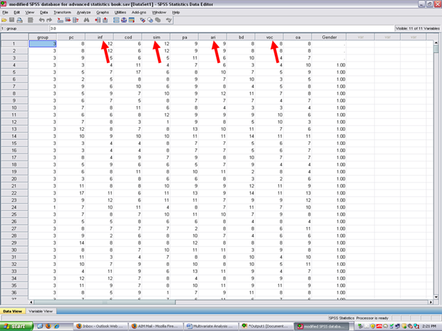
For this particular chapter, the research question on which we will conduct a MANOVA will be: What is the difference in verbal aptitude among elementary reading groups? Verbal aptitude consists of Verbal 1 (inf), Verbal 2 (sim), Verbal 3 (ari), and Verbal 4 (voc).

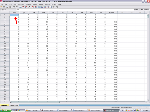
In this example, our independent or grouping variable is elementary reading group.

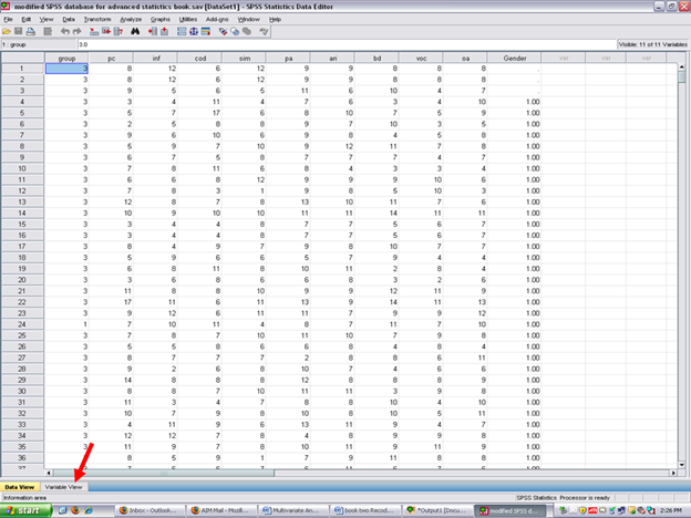
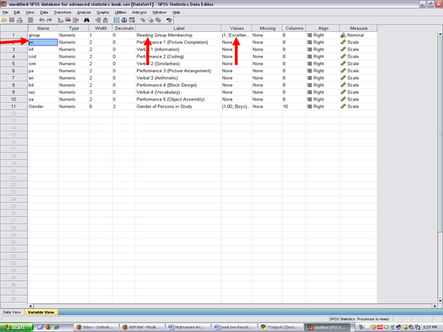
By clicking on variable view, you can see how many groups of students are present in the reading group variable; the names of the groups; and the numbers which have been assigned to each group.

After clicking on Variable View, the following screen will appear: Arrows have been placed toward the name of the independent or grouping variable; toward the label assigned to this variable; and then toward the values of each group.

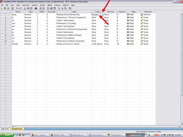
Now click on the cell for Reading Group Membership. Three dots will appear, indicating that another screen is beneath this one.

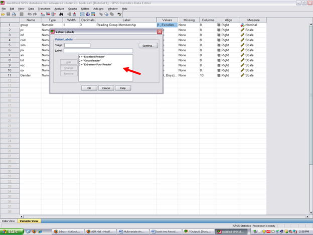
Click on the three dots shown in the screen above and the value and name of each of the reading groups will be shown. Our three groups are Excellent Reader (1), Good Reader (2), and Extremely Poor Reader (3).

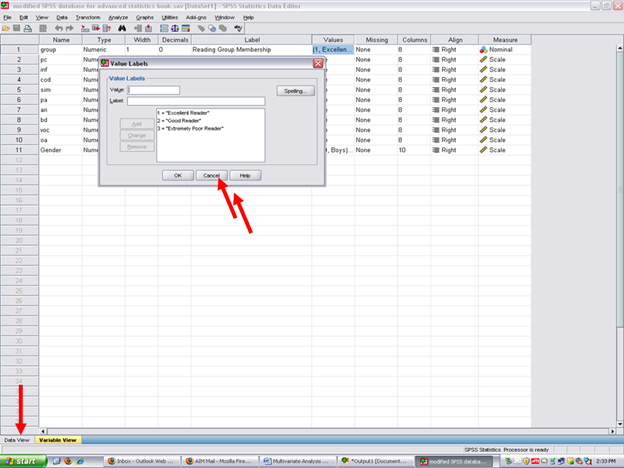
Now that you know what your independent (grouping) variable is and your dependent variables are, it is time to determine the extent to which the dependent variable data are normally distributed. Cancel out of the screen above. Then click on data view.

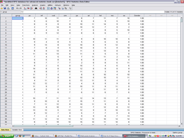
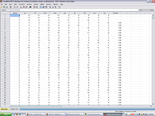
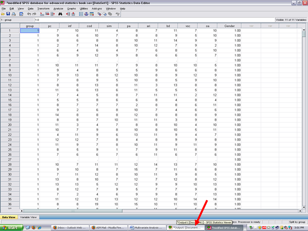
Your screen should now look like the one below.

Check for Skewness and Kurtosis values falling within/without the parameters of normality (-3 to +3). To do so, you need to obtain these values for each of your three groups for each of your four dependent variables.
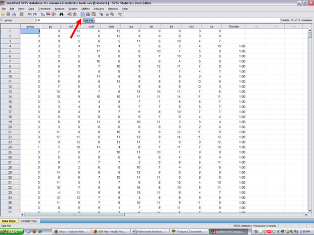
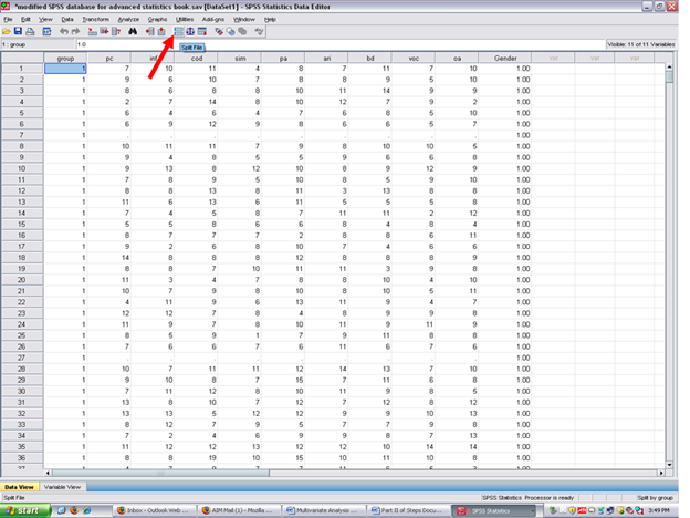
√ Split your file on the basis on your independent variable/fixed factor/grouping variable. To do so, click on the icon next to the scales. Holding your cursor on it will reveal Split File, as shown below.

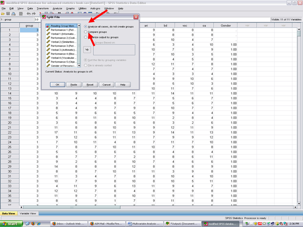
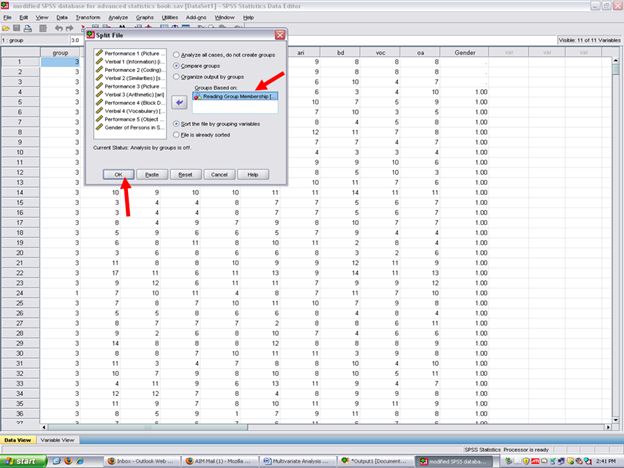
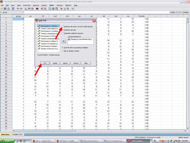
After clicking on the split file icon, the following screen will appear: You will note that the Analyze all cases, do not create groups is checked. This value is the default for SPSS as all cases are analyzed, unless otherwise specified. To obtain measures of normality for each of the three reading groups, the Compare groups button will need to be clicked.

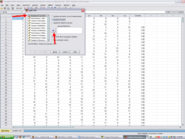
The screen below will appear after the Compare groups button has been clicked. Note that the Groups Based on rectangle has now become active. The independent (grouping) variable should be highlighted, as it already is, and then moved to the Groups Based on cell. After highlighting the Reading Group Membership variable, then click on the arrow below.

After clicking on the arrow, your independent variable of Reading Group Membership is now in the Groups Based on cell. Now click on OK.

Now all SPSS analyses will be calculated separately for each of the three reading groups.

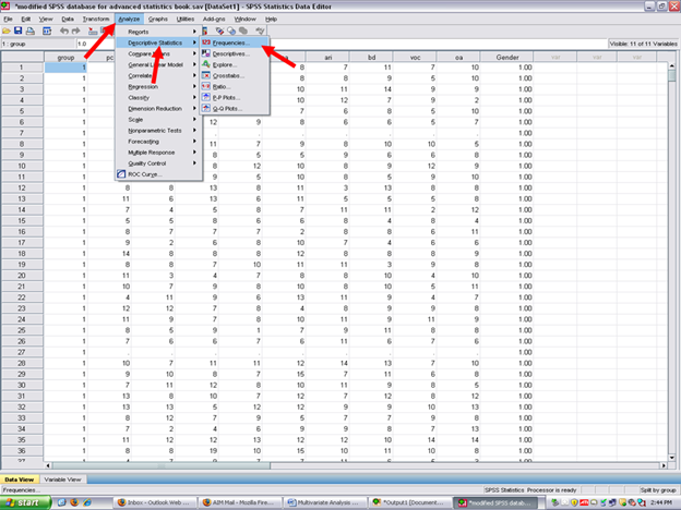
√ Analyze
* Descriptive Statistics
* Frequencies

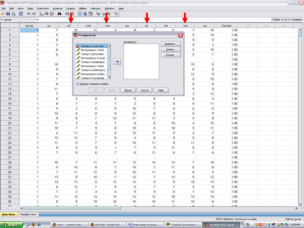
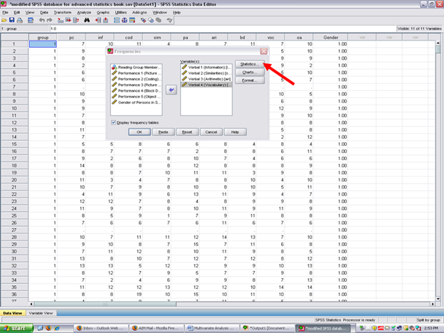
After clicking on frequencies, the following screen should now be present. Remember that the dependent variables in this example are Verbal 1 through Verbal 4 (i.e., inf, ari, voc)

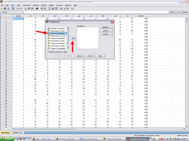
√ Move over the dependent variables. In this example, highlight each of the dependent variables one at a time and click on the right arrow.

When all four dependent variables are in the Variable cell, then click on Statistics.

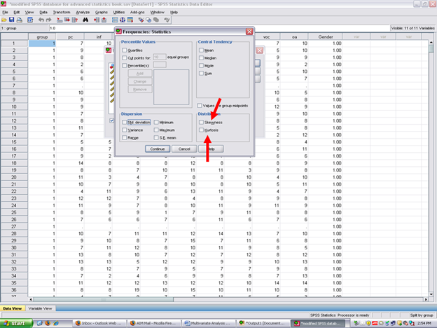
After clicking on statistics, the screen below will appear. Note that no statistics items are checked. For purposes of this example, only the skewness and kurtosis items will be checked. Although readers may obtain descriptive statistics at this screen, the MANOVA procedure itself can be used to obtain that information.

Though previously discussed in the steps and screenshots chapters for the basic statistical procedures, readers may find the following information helpful in understanding skewness and kurtosis and their importance for conducting statistical procedures.
* Skewness [Note. Skewness refers to the extent to which the data are normally distributed around the mean. Skewed data involve having either mostly high scores with a few low ones or having mostly low scores with a few high ones.] Readers are referred to the following sources for a more detailed definition of skewness: http://www.statistics.com/index.php?page=glossary&term_id=356 and http://www.statsoft.com/textbook/basic-statistics/#Descriptive%20statisticsb
To standardize the skewness value so that its value can be constant across datasets and across studies, the following calculation must be made: Take the skewness value from the SPSS output and divide it by the Std. error of skewness. If the resulting calculation is within -3 to +3, then the skewness of the dataset is within the range of normality (Onwuegbuzie & Daniel, 2002). If the resulting calculation is outside of this +/-3 range, the dataset is not normally distributed.
* Kurtosis [Note. Kurtosis also refers to the extent to which the data are normally distributed around the mean. This time, the data are piled up higher than normal around the mean or piled up higher than normal at the ends of the distribution.] Readers are referred to the following sources for a more detailed definition of kurtosis: http://www.statistics.com/index.php?page=glossary&term_id=326 and http://www.statsoft.com/textbook/basic-statistics/#Descriptive%20statisticsb
To standardize the kurtosis value so that its value can be constant across datasets and across studies, the following calculation must be made: Take the kurtosis value from the SPSS output and divide it by the Std. error of kurtosis. If the resulting calculation is within -3 to +3, then the kurtosis of the dataset is within the range of normality (Onwuegbuzie & Daniel, 2002). If the resulting calculation is outside of this +/-3 range, the dataset is not normally distributed. Then the kurtosis of the dataset is within the range of normality (Onwuegbuzie & Daniel, 2002). If the resulting calculation is outside of this +/-3 range, the dataset is not normally distributed.
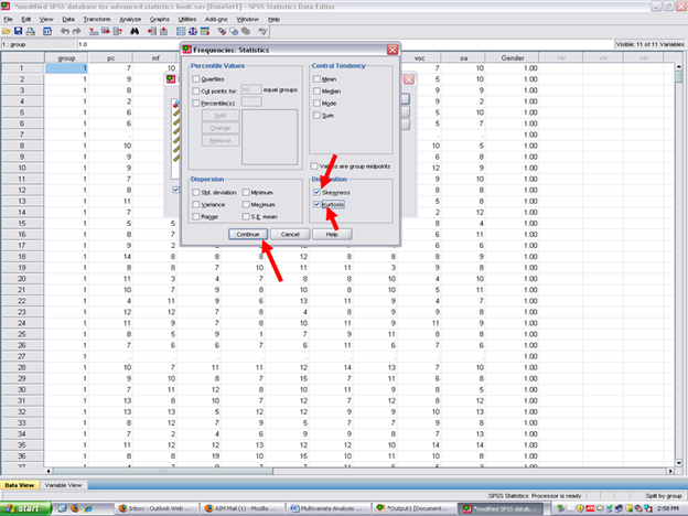
Click on Skewness, Kurtosis, and Continue

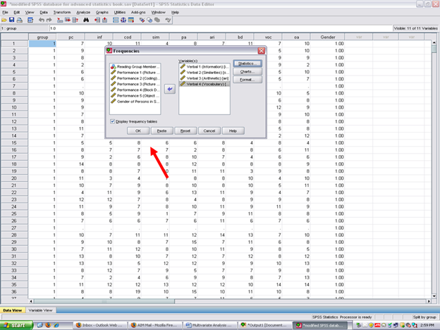
Now click on OK.

If SPSS does not send you to the Output screen, click on the Output button at the bottom of your screen so that you can view the results of the statistics you just had SPSS calculate for you.

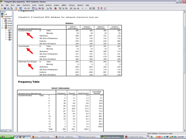
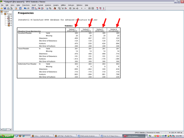
Clicking on the Output icon will result in the screen below being present. You will note that the Statistics table below contains statistics for the Excellent Reader group; for the Good Reader group; and for the Extremely Poor Reader group.

In the columns to the right of the three reading groups are the skewness and kurtosis values for the four dependent variables.

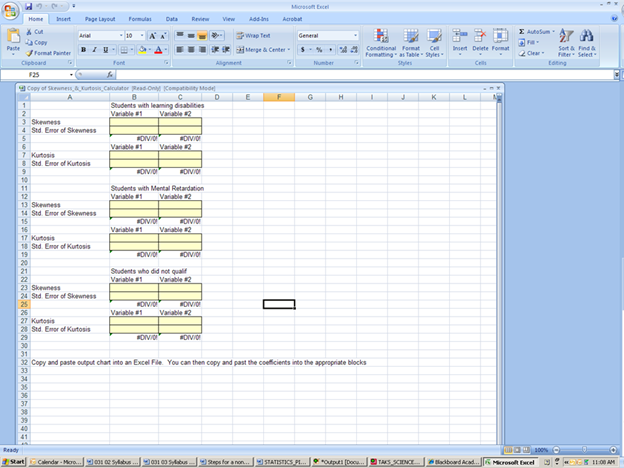
Using the skewness and kurtosis value for each dependent variable above for each of the three groups above, type them in one at a time into the standardized coefficients calculator. To be regarded as being normally distributed, the coefficient should be within -3 to +3 (Onwuegbuzie & Daniel, 2002).

After calculating the standardized coefficients, record the number that are within +/-3 and the number that are outside of these boundaries. This information needs to be discussed in your results section where you document your checks of the assumptions underlying this particular statistical technique.
Now, before conducting the MANOVA to answer our research question, this dataset must be put back together. Remember that the dataset is currently split. As you were in the SPSS Output screen, make sure that you go back to the Data screen before continuing.
To unsplit the file,
√ Split Files (the icon next to the scales)

Clicking on split files will reveal this screen. Although two ways exist in which to have SPSS analyze all cases, the easiest is simply to click on:
√ Analyze all cases, do not create groups
Then, √ OK

After clicking on OK, your screen should now look like the one below.
