7.1 The Central Limit Theorem1
7.1.1 Student Learning Outcomes
By the end of this chapter, the student should be able to:
• Recognize the Central Limit Theorem problems.
• Classify continuous word problems by their distributions.
• Apply and interpret the Central Limit Theorem for Means.
• Apply and interpret the Central Limit Theorem for Sums.
7.1.2 Introduction
Why are we so concerned with means? Two reasons are that they give us a middle ground for comparison
and they are easy to calculate. In this chapter, you will study means and the Central Limit Theorem.
The Central Limit Theorem (CLT for short) is one of the most powerful and useful ideas in all of statistics.
Both alternatives are concerned with drawing finite samples of size n from a population with a known
mean, µ, and a known standard deviation, σ. The first alternative says that if we collect samples of size
n and n is "large enough," calculate each sample’s mean, and create a histogram of those means, then the
resulting histogram will tend to have an approximate normal bell shape. The second alternative says that
if we again collect samples of size n that are "large enough," calculate the sum of each sample and create a
histogram, then the resulting histogram will again tend to have a normal bell-shape.
In either case, it does not matter what the distribution of the original population is, or whether you even
need to know it. The important fact is that the sample means and the sums tend to follow the normal
distribution. And, the rest you will learn in this chapter.
The size of the sample, n, that is required in order to be to be ’large enough’ depends on the original
population from which the samples are drawn. If the original population is far from normal then more
observations are needed for the sample means or the sample sums to be normal. Sampling is done with
replacement.
Optional Collaborative Classroom Activity
1This content is available online at <http://cnx.org/content/m16953/1.17/>.
279
280
CHAPTER 7. THE CENTRAL LIMIT THEOREM
Do the following example in class: Suppose 8 of you roll 1 fair die 10 times, 7 of you roll 2 fair dice 10
times, 9 of you roll 5 fair dice 10 times, and 11 of you roll 10 fair dice 10 times.
Each time a person rolls more than one die, he/she calculates the sample mean of the faces showing. For
example, one person might roll 5 fair dice and get a 2, 2, 3, 4, 6 on one roll.
The mean is
2+2+3+4+6 = 3.4.
The 3.4 is one mean when 5 fair dice are rolled. This same person would
5
roll the 5 dice 9 more times and calculate 9 more means for a total of 10 means.
Your instructor will pass out the dice to several people as described above. Roll your dice 10 times. For
each roll, record the faces and find the mean. Round to the nearest 0.5.
Your instructor (and possibly you) will produce one graph (it might be a histogram) for 1 die, one graph for
2 dice, one graph for 5 dice, and one graph for 10 dice. Since the "mean" when you roll one die, is just the
face on the die, what distribution do these means appear to be representing?
Draw the graph for the means using 2 dice. Do the sample means show any kind of pattern?
Draw the graph for the means using 5 dice. Do you see any pattern emerging?
Finally, draw the graph for the means using 10 dice. Do you see any pattern to the graph? What can you
conclude as you increase the number of dice?
As the number of dice rolled increases from 1 to 2 to 5 to 10, the following is happening:
1. The mean of the sample means remains approximately the same.
2. The spread of the sample means (the standard deviation of the sample means) gets smaller.
3. The graph appears steeper and thinner.
You have just demonstrated the Central Limit Theorem (CLT).
The Central Limit Theorem tells you that as you increase the number of dice, the sample means tend
toward a normal distribution (the sampling distribution).
7.2 The Central Limit Theorem for Sample Means (Averages)2
Suppose X is a random variable with a distribution that may be known or unknown (it can be any distri-
bution). Using a subscript that matches the random variable, suppose:
a. µ X = the mean of X
b. σ X = the standard deviation of X
If you draw random samples of size n, then as n increases, the random variable X which consists of sample
means, tends to be normally distributed and
X ∼ N µ X, σ X
√n
The Central Limit Theorem for Sample Means says that if you keep drawing larger and larger samples
(like rolling 1, 2, 5, and, finally, 10 dice) and calculating their means the sample means form their own
normal distribution (the sampling distribution). The normal distribution has the same mean as the
original distribution and a variance that equals the original variance divided by n, the sample size. n is the
number of values that are averaged together not the number of times the experiment is done.
2This content is available online at <http://cnx.org/content/m16947/1.23/>.
281
To put it more formally, if you draw random samples of size n,the distribution of the random vari-
able X, which consists of sample means, is called the sampling distribution of the mean. The sampling
distribution of the mean approaches a normal distribution as n, the sample size, increases.
The random variable X has a different z-score associated with it than the random variable X. x is the value
of X in one sample.
x − µ
z =
X
(7.1)
σ X
√n
µ X is both the average of X and of X.
σ
= σ X
√
= standard deviation of X and is called the standard error of the mean.
X
n
Example 7.1
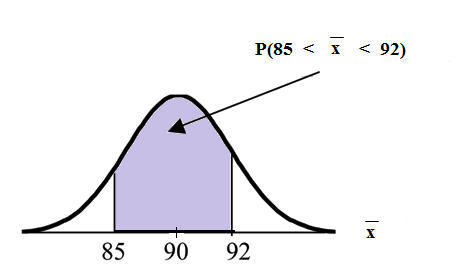
An unknown distribution has a mean of 90 and a standard deviation of 15. Samples of size n = 25
are drawn randomly from the population.
Problem 1
Find the probability that the sample mean is between 85 and 92.
Solution
Let X = one value from the original unknown population. The probability question asks you to
find a probability for the sample mean.
Let X = the mean of a sample of size 25. Since µ X = 90, σ X = 15, and n = 25;
then X ∼ N 90, 15
√25
Find P (85 < x < 92)
Draw a graph.
P (85 < x < 92) = 0.6997
The probability that the sample mean is between 85 and 92 is 0.6997.
TI-83 or 84: ♥♦r♠❛❧❝❞❢(lower value, upper value, mean, standard error of the mean)
The parameter list is abbreviated (lower value, upper value, µ, σ
√ )
n
♥♦r♠❛❧❝❞❢ 85, 92, 90, 15
√
= 0.6997
25
282
CHAPTER 7. THE CENTRAL LIMIT THEOREM
Problem 2
Find the value that is 2 standard deviations above the expected value (it is 90) of the sample mean.
Solution
To find the value that is 2 standard deviations above the expected value 90, use the formula
value = µ X + (#ofSTDEVs) σ X
√n
value = 90 + 2 · 15
√
= 96
25
So, the value that is 2 standard deviations above the expected value is 96.
Example 7.2
The length of time, in hours, it takes an "over 40" group of people to play one soccer match is
normally distributed with a mean of 2 hours and a standard deviation of 0.5 hours. A sample of
size n = 50 is drawn randomly from the population.
Problem
Find the probability that the sample mean is between 1.8 hours and 2.3 hours.
Solution
Let X = the time, in hours, it takes to play one soccer match.
The probability question asks you to find a probability for the sample mean time, in hours, it
takes to play one soccer match.
Let X = the mean time, in hours, it takes to play one soccer match.
If µ X = _________, σ X = __________, and n = ___________, then X ∼ N(______, ______)
by the Central Limit Theorem for Means.
µ X = 2, σ X = 0.5, n = 50, and X ∼ N 2 , 0.5
√50
Find P (1.8 < x < 2.3).
Draw a graph.
P (1.8 < x < 2.3) = 0.9977
♥♦r♠❛❧❝❞❢ 1.8, 2.3, 2, .5
√
= 0.9977
50
The probability that the mean time is between 1.8 hours and 2.3 hours is ______.
283
7.3 The Central Limit Theorem for Sums3
Suppose X is a random variable with a distribution that may be known or unknown (it can be any distri-
bution) and suppose:
a. µ X = the mean of X
b. σ X = the standard deviation of X
If you draw random samples of size n, then as n increases, the random variable ΣX which consists of sums
tends to be normally distributed and
√
ΣX ∼ N n · µ X, n · σ X
The Central Limit Theorem for Sums says that if you keep drawing larger and larger samples and taking
their sums, the sums form their own normal distribution (the sampling distribution) which approaches a
normal distribution as the sample size increases. The normal distribution has a mean equal to the original
mean multiplied by the sample size and a standard deviation equal to the original standard deviation
multiplied by the square root of the sample size.
The random variable ΣX has the following z-score associated with it:
a. Σx is one sum.
Σ
b. z = x−n· µ X
√n· σ X
a. n · µ X = the mean of ΣX
√
b.
n · σ X = standard deviation of ΣX
Example 7.3
An unknown distribution has a mean of 90 and a standard deviation of 15. A sample of size 80 is
drawn randomly from the population.
Problem
a. Find the probability that the sum of the 80 values (or the total of the 80 values) is more than
7500.
b. Find the sum that is 1.5 standard deviations above the mean of the sums.
Solution
Let X = one value from the original unknown population. The probability question asks you to
find a probability for the sum (or total of) 80 values.
ΣX = the sum or total of 80 values. Since µ X = 90, σ X = 15, and n = 80, then
√
ΣX ∼ N 80 · 90, 80 · 15
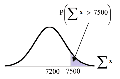
•. mean of the sums = n · µ X = (80) (90) = 7200
√
√
•. standard deviation of the sums =
n · σ X =
80 · 15
•. sum of 80 values = Σx = 7500
a: Find P (Σx > 7500)
3This content is available online at <http://cnx.org/content/m16948/1.16/>.
284
CHAPTER 7. THE CENTRAL LIMIT THEOREM
P (Σx > 7500) = 0.0127
♥♦r♠❛❧❝❞❢(lower value, upper value, mean of sums, st❞❡✈ of sums)
√
The parameter list is abbreviated (lower, upper, n · µ X, n · σ X)
√
♥♦r♠❛❧❝❞❢(7500,1E99, 80 · 90, 80 · 15 = 0.0127
Reminder: 1E99 = 1099. Press the ❊❊ key for E.
b: Find Σx where z = 1.5:
√
√
Σx = n · µ X + z · n · σ X = (80)(90) + (1.5)( 80) (15) = 7401.2
7.4 Using the Central Limit Theorem4
It is important for you to understand when to use the CLT. If you are being asked to find the probability of
the mean, use the CLT for the mean. If you are being asked to find the probability of a sum or total, use the
CLT for sums. This also applies to percentiles for means and sums.
NOTE: If you are being asked to find the probability of an individual value, do not use the CLT.
Use the distribution of its random variable.
7.4.1 Examples of the Central Limit Theorem
Law of Large Numbers
The Law of Large Numbers says that if you take samples of larger and larger size from any population,
then the mean x of the sample tends to get closer and closer to µ. From the Central Limit Theorem, we
know that as n gets larger and larger, the sample means follow a normal distribution. The larger n gets, the
smaller the standard deviation gets. (Remember that the standard deviation for X is σ
√
.) This means that
n
the sample mean x must be close to the population mean µ. We can say that µ is the value that the sample
means approach as n gets larger. The Central Limit Theorem illustrates the Law of Large Numbers.
Central Limit Theorem for the Mean and Sum Examples
4This content is available online at <http://cnx.org/content/m16958/1.21/>.
285
Example 7.4
A study involving stress is done on a college campus among the students. The stress scores follow
a uniform distribution with the lowest stress score equal to 1 and the highest equal to 5. Using a
sample of 75 students, find:
1. The probability that the mean stress score for the 75 students is less than 2.
2. The 90th percentile for the mean stress score for the 75 students.
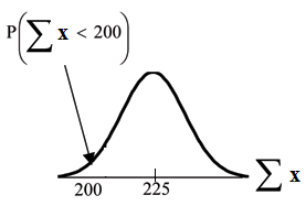
3. The probability that the total of the 75 stress scores is less than 200.
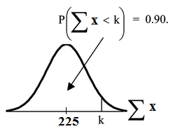
4. The 90th percentile for the total stress score for the 75 students.
Let X = one stress score.
Problems 1. and 2. ask you to find a probability or a percentile for a mean. Problems 3 and 4 ask
you to find a probability or a percentile for a total or sum. The sample size, n, is equal to 75.
Since the individual stress scores follow a uniform distribution, X ∼ U (1, 5) where a = 1 and
b = 5 (See Continuous Random Variables5 for the uniform).
µ X = a+b = 1+5 = 3
2
2
σ X =
(b−a)2 =
(5−1)2 = 1.15
12
12
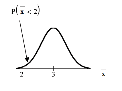
For problems 1. and 2., let X = the mean stress score for the 75 students. Then,
X ∼ N 3, 1.15
√
where n = 75.
75
Problem 1
Find P (x < 2).
Draw the graph.
Solution
P (x < 2) = 0
The probability that the mean stress score is less than 2 is about 0.
♥♦r♠❛❧❝❞❢ 1, 2, 3, 1.15
√
= 0
75
REMINDER: The smallest stress score is 1. Therefore, the smallest mean for 75 stress scores is 1.
5"Continuous Random Variables: Introduction" <http://cnx.org/content/m16808/latest/>
286
CHAPTER 7. THE CENTRAL LIMIT THEOREM
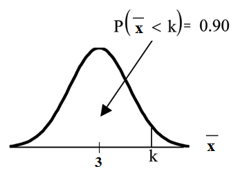
Problem 2
Find the 90th percentile for the mean of 75 stress scores. Draw a graph.
Solution
Let k = the 90th precentile.
Find k where P (x < k) = 0.90.
k = 3.2
The 90th percentile for the mean of 75 scores is about 3.2. This tells us that 90% of all the means of
75 stress scores are at most 3.2 and 10% are at least 3.2.
✐♥✈◆♦r♠ .90, 3, 1.15
√
= 3.2
75
For problems c and d, let ΣX = the sum of the 75 stress scores.
Then, ΣX ∼
√
N (75) · (3) ,
75 · 1.15
Problem 3
Find P (Σx < 200).
Draw the graph.
Solution
The mean of the sum of 75 stress scores is 75 · 3 = 225
√
The standard deviation of the sum of 75 stress scores is
75 · 1.15 = 9.96
P (Σx < 200) = 0
287
The probability that the total of 75 scores is less than 200 is about 0.
√
♥♦r♠❛❧❝❞❢ 75, 200, 75 · 3, 75 · 1.15 = 0.
REMINDER: The smallest total of 75 stress scores is 75 since the smallest single score is 1.
Problem 4
Find the 90th percentile for the total of 75 stress scores. Draw a graph.
Solution
Let k = the 90th percentile.
Find k where P (Σx < k) = 0.90.
k = 237.8
The 90th percentile for the sum of 75 scores is about 237.8. This tells us that 90% of all the sums of
75 scores are no more than 237.8 and 10% are no less than 237.8.
√
✐♥✈◆♦r♠ .90, 75 · 3, 75 · 1.15 = 237.8
Example 7.5
Suppose that a market research analyst for a cell phone company conducts a study of their cus-
tomers who exceed the time allowance included on their basic cell phone contract; the analyst
finds that for those people who exceed the time included in their basic contract, the excess time
used follows an exponential distribution with a mean of 22 minutes.
Consider a random sample of 80 customers who exceed the time allowance included in their basic
cell phone contract.
Let X = the excess time used by one INDIVIDUAL cell phone customer who exceeds his contracted
time allowance.
X ∼ Exp
1
From Chapter 5, we know that
22
µ = 22 and σ = 22.
Let X = the mean excess time used by a sample of n = 80 customers who exceed their contracted
time allowance.
288
CHAPTER 7. THE CENTRAL LIMIT THEOREM
X ∼ N 22, 22
√
by the CLT for Sample Means
80
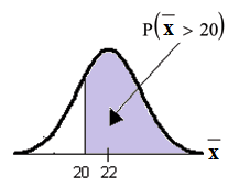
Problem 1
Using the CLT to find Probability:
a. Find the probability that the mean excess time used by the 80 customers in the sample is longer
than 20 minutes. This is asking us to find P (x > 20)
Draw the graph.
b. Suppose that one customer who exceeds the time limit for his cell phone contract is randomly
selected. Find the probability that this individual customer’s excess time is longer than 20
minutes. This is asking us to find P (x > 20)
c. Explain why the probabilities in (a) and (b) are different.
Solution
Part a.
Find: P (x > 20)
P (x > 20) = 0.7919 using ♥♦r♠❛❧❝❞❢ 20, 1E99, 22, 22
√80
The probability is 0.7919 that the mean excess time used is more than 20 minutes, for a sample of
80 customers who exceed their contracted time allowance.
REMINDER: 1E99 = 1099 and−1E99 = −1099. Press the ❊❊ key for E. Or just use 10^99 instead of
1E99.
Part b.
Find P(x>20) . Remember to use the exponential distribution for an individual: X∼Exp(1/22).
P(X>20) = e^(–(1/22)*20) or e^(–.04545*20) = 0.4029
Part c. Explain why the probabilities in (a) and (b) are different.
P (x > 20) = 0.4029 but P (x > 20) = 0.7919
The probabilities are not equal because we use different distributions to calculate the probability
for individuals and for means.
When asked to find the probability of an individual value, use the stated distribution of its ran-
dom variable; do not use the CLT. Use the CLT with the normal distribution when you are
being asked to find the probability for an mean.
289
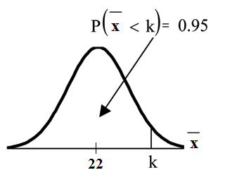
Problem 2
Using the CLT to find Percentiles:
Find the 95th percentile for the sample mean excess time for samples of 80 customers who exceed
their basic contract time allowances. Draw a graph.
Solution
Let k = the 95th percentile. Find k where P (x < k) = 0.95
k = 26.0 using ✐♥✈◆♦r♠ .95, 22, 22
√
= 26.0
80
The 95th percentile for the sample mean excess time used is about 26.0 minutes for random
samples of 80 customers who exceed their contractual allowed time.
95% of such samples would have means under 26 minutes; only 5% of such samples would have
means above 26 minutes.
NOTE: (HISTORICAL): Normal Approximation to the Binomial
Historically, being able to compute binomial probabilities was one of the most important applications of the
Central Limit Theorem. Binomial probabilities were displayed in a table in a book with a small value for n
(say, 20). To calculate the probabilities with large values of n, you had to use the binomial formula which
could be very complicated. Using the Normal Approximation to the Binomial simplified the process. To
compute the Normal Approximation to the Binomial, take a simple random sample from a population. You
must meet the conditions for a binomial distribution:
•. there are a certain number n of independent trials
•. the outcomes of any trial are success or failure
•. each trial has the same probability of a success p
Recall that if X is the binomial random variable, then X∼B (n, p). The shape of the binomial distribution
needs to be similar to the shape of the normal distribution. To ensure this, th