8.1 Confidence Intervals1
8.1.1 Student Learning Outcomes
By the end of this chapter, the student should be able to:
• Calculate and interpret confidence intervals for one population mean and one population proportion.
• Interpret the student-t probability distribution as the sample size changes.
• Discriminate between problems applying the normal and the student-t distributions.
8.1.2 Introduction
Suppose you are trying to determine the mean rent of a two-bedroom apartment in your town. You might
look in the classified section of the newspaper, write down several rents listed, and average them together.
You would have obtained a point estimate of the true mean. If you are trying to determine the percent of
times you make a basket when shooting a basketball, you might count the number of shots you make and
divide that by the number of shots you attempted. In this case, you would have obtained a point estimate
for the true proportion.
We use sample data to make generalizations about an unknown population. This part of statistics is called
inferential statistics. The sample data help us to make an estimate of a population parameter. We realize
that the point estimate is most likely not the exact value of the population parameter, but close to it. After
calculating point estimates, we construct confidence intervals in which we believe the parameter lies.
In this chapter, you will learn to construct and interpret confidence intervals. You will also learn a new
distribution, the Student’s-t, and how it is used with these intervals. Throughout the chapter, it is important
to keep in mind that the confidence interval is a random variable. It is the parameter that is fixed.
If you worked in the marketing department of an entertainment company, you might be interested in the
mean number of compact discs (CD’s) a consumer buys per month. If so, you could conduct a survey
and calculate the sample mean, x, and the sample standard deviation, s. You would use x to estimate
the population mean and s to estimate the population standard deviation. The sample mean, x, is the
point estimate for the population mean, µ. The sample standard deviation, s, is the point estimate for the
population standard deviation, σ.
1This content is available online at <http://cnx.org/content/m16967/1.16/>.
317
318
CHAPTER 8. CONFIDENCE INTERVALS
Each of x and s is also called a statistic.
A confidence interval is another type of estimate but, instead of being just one number, it is an interval
of numbers. The interval of numbers is a range of values calculated from a given set of sample data. The
confidence interval is likely to include an unknown population parameter.
Suppose for the CD example we do not know the population mean µ but we do know that the population
standard deviation is σ = 1 and our sample size is 100. Then by the Central Limit Theorem, the standard
deviation for the sample mean is
σ
√
=
1
√
= 0.1.
n
100
The Empirical Rule, which applies to bell-shaped distributions, says that in approximately 95% of the
samples, the sample mean, x, will be within two standard deviations of the population mean µ. For our CD
example, two standard deviations is (2) (0.1) = 0.2. The sample mean x is likely to be within 0.2 units of
µ.
Because x is within 0.2 units of µ, which is unknown, then µ is likely to be within 0.2 units of x in 95%
of the samples. The population mean µ is contained in an interval whose lower number is calculated by
taking the sample mean and subtracting two standard deviations ((2) (0.1)) and whose upper number is
calculated by taking the sample mean and adding two standard deviations. In other words, µ is between
x − 0.2 and x + 0.2 in 95% of all the samples.
For the CD example, suppose that a sample produced a sample mean x = 2. Then the unknown population
mean µ is between
x − 0.2 = 2 − 0.2 = 1.8 and x + 0.2 = 2 + 0.2 = 2.2
We say that we are 95% confident that the unknown population mean number of CDs is between 1.8 and
2.2. The 95% confidence interval is (1.8, 2.2).
The 95% confidence interval implies two possibilities. Either the interval (1.8, 2.2) contains the true mean µ
or our sample produced an x that is not within 0.2 units of the true mean µ. The second possibility happens
for only 5% of all the samples (100% - 95%).
Remember that a confidence interval is created for an unknown population parameter like the population
mean, µ. Confidence intervals for some parameters have the form
(point estimate - margin of error, point estimate + margin of error)
The margin of error depends on the confidence level or percentage of confidence.
When you read newspapers and journals, some reports will use the phrase "margin of error." Other reports
will not use that phrase, but include a confidence interval as the point estimate + or - the margin of error.
These are two ways of expressing the same concept.
NOTE: Although the text only covers symmetric confidence intervals, there are non-symmetric
confidence intervals (for example, a confidence interval for the standard deviation).
8.1.3 Optional Collaborative Classroom Activity
Have your instructor record the number of meals each student in your class eats out in a week. Assume
that the standard deviation is known to be 3 meals. Construct an approximate 95% confidence interval for
the true mean number of meals students eat out each week.
319
1. Calculate the sample mean.
2. σ = 3 and n = the number of students surveyed.
3. Construct the interval x − 2 · σ
√ , x + 2 · σ
√
n
n
We say we are approximately 95% confident that the true average number of meals that students eat out in
a week is between __________ and ___________.
8.2 Confidence Interval, Single Population Mean, Population Standard
Deviation Known, Normal2
8.2.1 Calculating the Confidence Interval
To construct a confidence interval for a single unknown population mean µ , where the population stan-
dard deviation is known, we need x as an estimate for µ and we need the margin of error. Here, the
margin of error is called the error bound for a population mean (abbreviated EBM). The sample mean x is
the point estimate of the unknown population mean µ
The confidence interval estimate will have the form:
(point estimate - error bound, point estimate + error bound) or, in symbols,(x − EBM, x + EBM)
The margin of error depends on the confidence level (abbreviated CL). The confidence level is often con-
sidered the probability that the calculated confidence interval estimate will contain the true population
parameter. However, it is more accurate to state that the confidence level is the percent of confidence in-
tervals that contain the true population parameter when repeated samples are taken. Most often, it is the
choice of the person constructing the confidence interval to choose a confidence level of 90% or higher
because that person wants to be reasonably certain of his or her conclusions.
There is another probability called alpha ( α). α is related to the confidence level CL. α is the probability that the interval does not contain the unknown population parameter.
Mathematically, α + CL = 1.
Example 8.1
Suppose we have collected data from a sample. We know the sample mean but we do not know
the mean for the entire population.
The sample mean is 7 and the error bound for the mean is 2.5.
x = 7 and EBM = 2.5.
The confidence interval is (7 − 2.5, 7 + 2.5); calculating the values gives (4.5, 9.5).
If the confidence level (CL) is 95%, then we say that "We estimate with 95% confidence that the
true value of the population mean is between 4.5 and 9.5."
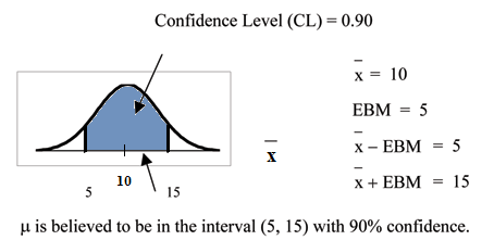
A confidence interval for a population mean with a known standard deviation is based on the fact that the
sample means follow an approximately normal distribution. Suppose that our sample has a mean of x = 10
and we have constructed the 90% confidence interval (5, 15) where EBM = 5.
To get a 90% confidence interval, we must include the central 90% of the probability of the normal distri-
bution. If we include the central 90%, we leave out a total of α = 10% in both tails, or 5% in each tail, of the
normal distribution.
2This content is available online at <http://cnx.org/content/m16962/1.23/>.
320
CHAPTER 8. CONFIDENCE INTERVALS
To capture the central 90%, we must go out 1.645 "standard deviations" on either side of the calculated
sample mean. 1.645 is the z-score from a Standard Normal probability distribution that puts an area of 0.90
in the center, an area of 0.05 in the far left tail, and an area of 0.05 in the far right tail.
It is important that the "standard deviation" used must be appropriate for the parameter we are estimating.
So in this section, we need to use the standard deviation that applies to sample means, which is σ
√
. σ
√
is
n
n
commonly called the "standard error of the mean" in order to clearly distinguish the standard deviation for
a mean from the population standard deviation σ.
In summary, as a result of the Central Limit Theorem:
• X is normally distributed, that is, X ∼ N µ X, σ
√
.
n
•
When the population standard deviation σ is known, we use a Normal distribution to calculate
the error bound.
Calculating the Confidence Interval:
To construct a confidence interval estimate for an unknown population mean, we need data from a random
sample. The steps to construct and interpret the confidence interval are:
• Calculate the sample mean x from the sample data. Remember, in this section, we already know the
population standard deviation σ.
• Find the Z-score that corresponds to the confidence level.
• Calculate the error bound EBM
• Construct the confidence interval
• Write a sentence that interprets the estimate in the context of the situation in the problem. (Explain
what the confidence interval means, in the words of the problem.)
We will first examine each step in more detail, and then illustrate the process with some examples.
Finding z for the stated Confidence Level
When we know the population standard deviation σ, we use a standard normal distribution to calculate
the error bound EBM and construct the confidence interval. We need to find the value of z that puts an area
equal to the confidence level (in decimal form) in the middle of the standard normal distribution Z∼N(0,1).
The confidence level, CL, is the area in the middle of the standard normal distribution. CL = 1 − α. So α is
the area that is split equally between the two tails. Each of the tails contains an area equal to α .
2
The z-score that has an area to the right of α is denoted by z
2
α
2
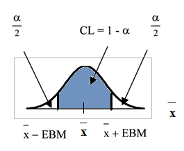
321
For example, when CL = 0.95 then α = 0.05 and α = 0.025 ; we write z = z
2
α
.025
2
The area to the right of z.025 is 0.025 and the area to the left of z.025 is 1-0.025 = 0.975
z α = z0.025 = 1.96 , using a calculator, computer or a Standard Normal probability table.
2
Using the TI83, TI83+ or TI84+ calculator: ✐♥✈◆♦r♠(0.975, 0, 1) = 1.96
CALCULATOR NOTE: Remember to use area to the LEFT of z α ; in this chapter the last two inputs in the
2
invNorm command are 0,1 because you are using a Standard Normal Distribution Z∼N(0,1)
EBM: Error Bound
The error bound formula for an unknown population mean µ when the population standard deviation σ is
known is
• EBM = z α · σ
√
2
n
Constructing the Confidence Interval
• The confidence interval estimate has the format (x − EBM, x + EBM).
The graph gives a picture of the entire situation.
CL + α + α = CL +
2
2
α = 1.
Writing the Interpretation
The interpretation should clearly state the confidence level (CL), explain what population parameter is
being estimated (here, a population mean), and should state the confidence interval (both endpoints). "We
estimate with ___% confidence that the true population mean (include context of the problem) is between
___ and ___ (include appropriate units)."
Example 8.2
Suppose scores on exams in statistics are normally distributed with an unknown population mean
and a population standard deviation of 3 points. A random sample of 36 scores is taken and gives
a sample mean (sample mean score) of 68. Find a confidence interval estimate for the population
mean exam score (the mean score on all exams).
Problem
Find a 90% confidence interval for the true (population) mean of statistics exam scores.
322
CHAPTER 8. CONFIDENCE INTERVALS
Solution
• You can use technology to directly calculate the confidence interval
• The first solution is shown step-by-step (Solution A).
• The second solution uses the TI-83, 83+ and 84+ calculators (Solution B).
Solution A
To find the confidence interval, you need the sample mean, x, and the EBM.
x = 68
EBM = z α ·
σ
√
2
n
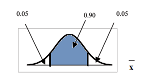
σ = 3 ; n = 36 ; The confidence level is 90% (CL=0.90)
CL = 0.90 so α = 1 − CL = 1 − 0.90 = 0.10
α = 0.05
z = z
2
α
.05
2
The area to the right of z.05 is 0.05 and the area to the left of z.05 is 1−0.05=0.95
z α = z.05 = 1.645
2
using invNorm(0.95,0,1) on the TI-83,83+,84+ calculators. This can also be found using appropriate
commands on other calculators, using a computer, or using a probability table for the Standard
Normal distribution.
EBM = 1.645 ·
3
√
= 0.8225
36
x − EBM = 68 − 0.8225 = 67.1775
x + EBM = 68 + 0.8225 = 68.8225
The 90% confidence interval is (67.1775, 68.8225).
Solution B
Using a function of the TI-83, TI-83+ or TI-84 calculators:
Press ❙❚❆❚ and arrow over to ❚❊❙❚❙.
Arrow down to ✼✿❩■♥t❡r✈❛❧.
Press ❊◆❚❊❘.
Arrow to ❙t❛ts and press ❊◆❚❊❘.
Arrow down and enter 3 for σ, 68 for x , 36 for n, and .90 for ❈✲❧❡✈❡❧.
Arrow down to ❈❛❧❝✉❧❛t❡ and press ❊◆❚❊❘.
The confidence interval is (to 3 decimal places) (67.178, 68.822).
Interpretation
We estimate with 90% confidence that the true population mean exam score for all statistics stu-
dents is between 67.18 and 68.82.
Explanation of 90% Confidence Level
90% of all confidence intervals constructed in this way contain the true mean statistics exam score.
For example, if we constructed 100 of these confidence intervals, we would expect 90 of them to
contain the true population mean exam score.
323
8.2.2 Changing the Confidence Level or Sample Size
Example 8.3: Changing the Confidence Level
Suppose we change the original problem by using a 95% confidence level. Find a 95% confidence
interval for the true (population) mean statistics exam score.
Solution
To find the confidence interval, you need the sample mean, x, and the EBM.
x = 68
EBM = z α ·
σ
√
2
n
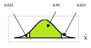
σ = 3 ; n = 36 ; The confidence level is 95% (CL=0.95)
CL = 0.95 so α = 1 − CL = 1 − 0.95 = 0.05
α = 0.025
z = z
2
α
.025
2
The area to the right of z.025 is 0.025 and the area to the left of z.025 is 1−0.025=0.975
z α = z.025 = 1.96
2
using invnorm(.975,0,1) on the TI-83,83+,84+ calculators. (This can also be found using appropri-
ate commands on other calculators, using a computer, or using a probability table for the Standard
Normal distribution.)
EBM = 1.96 ·
3
√
= 0.98
36
x − EBM = 68 − 0.98 = 67.02
x + EBM = 68 + 0.98 = 68.98
Interpretation
We estimate with 95 % confidence that the true population mean for all statistics exam scores is
between 67.02 and 68.98.
Explanation of 95% Confidence Level
95% of all confidence intervals constructed in this way contain the true value of the population
mean statistics exam score.
Comparing the results
The 90% confidence interval is (67.18, 68.82). The 95% confidence interval is (67.02, 68.98). The
95% confidence interval is wider. If you look at the graphs, because the area 0.95 is larger than the
area 0.90, it makes sense that the 95% confidence interval is wider.
324
CHAPTER 8. CONFIDENCE INTERVALS
(a)
(b)
Figure 8.1
Summary: Effect of Changing the Confidence Level
• Increasing the confidence level increases the error bound, making the confidence interval
wider.
• Decreasing the confidence level decreases the error bound, making the confidence interval
narrower.
Example 8.4: Changing the Sample Size:
Suppose we change the original problem to see what happens to the error bound if the sample size
is changed.
Problem
Leave everything the same except the sample size. Use the original 90% confidence level. What
happens to the error bound and the confidence interval if we increase the sample size and use
n=100 instead of n=36? What happens if we decrease the sample size to n=25 instead of n=36?
• x = 68
• EBM = z α ·
σ
√
2
n
• σ = 3 ; The confidence level is 90% (CL=0.90) ; z α = z.05 = 1.645
2
Solution A
If we increase the sample size n to 100, we decrease the error bound.
When n = 100 : EBM = z α ·
σ
√
= 1.645 ·
3
√
= 0.4935
2
n
100
Solution B
If we decrease the sample size n to 25, we increase the error bound.
When n = 25 : EBM = z α ·
σ
√
= 1.645 ·
3
√
= 0.987
2
n
25
Summary: Effect of Changing the Sample Size
• Increasing the sample size causes the error bound to decrease, making the confidence inter-
val narrower.
• Decreasing the sample size causes the error bound to increase, making the confidence inter-
val wider.
325
8.2.3 Working Backwards to Find the Error Bound or Sample Mean
Working Bacwards to find the Error Bound or the Sample Mean
When we calculate a confidence interval, we find the sample mean and calculate the error bound and use
them to calculate the confidence interval. But sometimes when we read statistical studies, the study may
state the confidence interval only. If we know the confidence interval, we can work backwards to find both
the error bound and the sample mean.
Finding the Error Bound
• From the upper value for the interval, subtract the sample mean
• OR, From the upper value for the interval, subtract the lower value. Then divide the difference by 2.
Finding the Sample Mean
• Subtract the error bound from the upper value of the confidence interval
• OR, Average the upper and lower endpoints of the confidence interval
Notice that there are two methods to perform each calculation. You can choose the method that is easier to
use with the information you know.
Example 8.5
Suppose we know that a confidence interval is (67.18, 68.82) and we want to find the error bound.
We may know that the sample mean is 68. Or perhaps our source only gave the confidence interval
and did not tell us the value of the the sample mean.
Calculate the Error Bound:
• If we know that the sample mean is 68: EBM = 68.82 − 68 = 0.82
• If we don’t know the sample mean: EBM = (68.82−67.18) = 0.82
2
Calculate the Sample Mean:
• If we know the error bound: x = 68.82 − 0.82 = 68
• If we don’t know the error bound: x = (67.18+68.82) = 68
2
8.2.4 Calculating the Sample Size n
If researchers desire a specific margin of error, then they can use the error bound formula to calculate the
required sample size.
The error bound formula for a population mean when the population standard deviation is known is
EBM = z α ·
σ
√
2
n
2
The formula for sample size is n = z2 σ , found by solving the error bound formula for n
EBM2<