Data, Two Proportions
10.1 Hypothesis Testing: Two Population Means and Two Population
Proportions1
10.1.1 Student Learning Outcomes
By the end of this chapter, the student should be able to:
• Classify hypothesis tests by type.
• Conduct and interpret hypothesis tests for two population means, population standard deviations
known.
• Conduct and interpret hypothesis tests for two population means, population standard deviations
unknown.
• Conduct and interpret hypothesis tests for two population proportions.
• Conduct and interpret hypothesis tests for matched or paired samples.
10.1.2 Introduction
Studies often compare two groups. For example, researchers are interested in the effect aspirin has in
preventing heart attacks. Over the last few years, newspapers and magazines have reported about various
aspirin studies involving two groups. Typically, one group is given aspirin and the other group is given a
placebo. Then, the heart attack rate is studied over several years.
There are other situations that deal with the comparison of two groups. For example, studies compare var-
ious diet and exercise programs. Politicians compare the proportion of individuals from different income
brackets who might vote for them. Students are interested in whether SAT or GRE preparatory courses
really help raise their scores.
In the previous chapter, you learned to conduct hypothesis tests on single means and single proportions.
You will expand upon that in this chapter. You will compare two means or two proportions to each other.
The general procedure is still the same, just expanded.
1This content is available online at <http://cnx.org/content/m17029/1.9/>.
419
CHAPTER 10. HYPOTHESIS TESTING: TWO MEANS, PAIRED DATA, TWO
420
PROPORTIONS
To compare two means or two proportions, you work with two groups. The groups are classified either as
independent or matched pairs. Independent groups mean that the two samples taken are independent,
that is, sample values selected from one population are not related in any way to sample values selected
from the other population. Matched pairs consist of two samples that are dependent. The parameter tested
using matched pairs is the population mean. The parameters tested using independent groups are either
population means or population proportions.
NOTE: This chapter relies on either a calculator or a computer to calculate the degrees of freedom,
the test statistics, and p-values. TI-83+ and TI-84 instructions are included as well as the test statis-
tic formulas. When using the TI-83+/TI-84 calculators, we do not need to separate two population
means, independent groups, population variances unknown into large and small sample sizes.
However, most statistical computer software has the ability to differentiate these tests.
This chapter deals with the following hypothesis tests:
Independent groups (samples are independent)
• Test of two population means.
• Test of two population proportions.
Matched or paired samples (samples are dependent)
• Becomes a test of one population mean.
10.2 Comparing Two Independent Population Means with Unknown
Population Standard Deviations2
1. The two independent samples are simple random samples from two distinct populations.
2. Both populations are normally distributed with the population means and standard deviations un-
known unless the sample sizes are greater than 30. In that case, the populations need not be normally
distributed.
NOTE: The test comparing two independent population means with unknown and possibly un-
equal population standard deviations is called the Aspin-Welch t-test. The degrees of freedom
formula was developed by Aspin-Welch.
The comparison of two population means is very common. A difference between the two samples depends
on both the means and the standard deviations. Very different means can occur by chance if there is great
variation among the individual samples. In order to account for the variation, we take the difference of
the sample means, X1 - X2 , and divide by the standard error (shown below) in order to standardize the
difference. The result is a t-score test statistic (shown below).
Because we do not know the population standard deviations, we estimate them using the two sample
standard deviations from our independent samples. For the hypothesis test, we calculate the estimated
standard deviation, or standard error, of the difference in sample means, X1 - X2.
The standard error is:
(S1)2
(S
+
2)2
(10.1)
n1
n2
The test statistic (t-score) is calculated as follows:
2This content is available online at <http://cnx.org/content/m17025/1.18/>.
421
t-score
(x1 − x2) − ( µ 1 − µ 2)
(10.2)
(S1)2 + (S2)2
n1
n2
where:
• s1 and s2, the sample standard deviations, are estimates of σ 1 and σ 2, respectively.
• σ 1 and σ 2 are the unknown population standard deviations.
• x1 and x2 are the sample means. µ 1 and µ 2 are the population means.
The degrees of freedom (df) is a somewhat complicated calculation. However, a computer or calculator cal-
culates it easily. The dfs are not always a whole number. The test statistic calculated above is approximated
by the student’s-t distribution with dfs as follows:
Degrees of freedom
2
(s1)2 + (s2)2
n1
n2
d f =
(10.3)
2
2
1
· (s1)2
+
1
· (s2)2
n1−1
n1
n2−1
n2
When both sample sizes n1 and n2 are five or larger, the student’s-t approximation is very good. Notice that
the sample variances s 2
2
1 and s2 are not pooled. (If the question comes up, do not pool the variances.)
NOTE: It is not necessary to compute this by hand. A calculator or computer easily computes it.
Example 10.1: Independent groups
The average amount of time boys and girls ages 7 through 11 spend playing sports each day is
believed to be the same. An experiment is done, data is collected, resulting in the table below.
Both populations have a normal distribution.
Sample Size
Average Number of
Sample Standard
Hours Playing Sports
Deviation
Per Day
√
Girls
9
2 hours
0.75
Boys
16
3.2 hours
1.00
Table 10.1
Problem
Is there a difference in the mean amount of time boys and girls ages 7 through 11 play sports each
day? Test at the 5% level of significance.
Solution
The population standard deviations are not known. Let g be the subscript for girls and b be the
subscript for boys. Then, µ g is the population mean for girls and µ b is the population mean for
boys. This is a test of two independent groups, two population means.
Random variable: Xg − Xb = difference in the sample mean amount of time girls and boys play
sports each day.
Ho: µ g = µ b
µ g − µ b = 0
CHAPTER 10. HYPOTHESIS TESTING: TWO MEANS, PAIRED DATA, TWO
422
PROPORTIONS
Ha: µ g = µ b
µ g − µ b = 0
The words "the same" tell you Ho has an "=". Since there are no other words to indicate Ha, then
assume "is different." This is a two-tailed test.
Distribution for the test: Use td f where d f is calculated using the d f formula for independent
groups, two population means. Using a calculator, d f is approximately 18.8462. Do not pool the
variances.
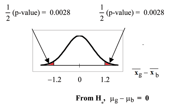
Calculate the p-value using a student’s-t distribution: p-value = 0.0054
Graph:
Figure 10.1
√
sg =
0.75
sb = 1
So, xg − xb = 2 − 3.2 = −1.2
Half the p-value is below -1.2 and half is above 1.2.
Make a decision: Since α > p-value, reject Ho.
This means you reject µ g = µ b. The means are different.
Conclusion: At the 5% level of significance, the sample data show there is sufficient evidence to
conclude that the mean number of hours that girls and boys aged 7 through 11 play sports per day
is different (mean number of hours boys aged 7 through 11 play sports per day is greater than the
mean number of hours played by girls OR the mean number of hours girls aged 7 through 11 play
sports per day is greater than the mean number of hours played by boys).
NOTE: TI-83+ and TI-84: Press ❙❚❆❚. Arrow over to ❚❊❙❚❙ and press ✹✿✷✲❙❛♠♣❚❚❡st. Arrow over
√
to Stats and press ❊◆❚❊❘. Arrow down and enter ✷ for the first sample mean,
0.75 for Sx1, ✾
for n1, ✸✳✷ for the second sample mean, ✶ for Sx2, and ✶✻ for n2. Arrow down to µ 1: and arrow
to ❞♦❡s ♥♦t ❡q✉❛❧ µ 2. Press ❊◆❚❊❘. Arrow down to Pooled: and ◆♦. Press ❊◆❚❊❘. Arrow down to
❈❛❧❝✉❧❛t❡ and press ❊◆❚❊❘. The p-value is p = 0.0054, the dfs are approximately 18.8462, and the
test statistic is -3.14. Do the procedure again but instead of Calculate do Draw.
423
Example 10.2
A study is done by a community group in two neighboring colleges to determine which one grad-
uates students with more math classes. College A samples 11 graduates. Their average is 4 math
classes with a standard deviation of 1.5 math classes. College B samples 9 graduates. Their aver-
age is 3.5 math classes with a standard deviation of 1 math class. The community group believes
that a student who graduates from college A has taken more math classes, on the average. Both
populations have a normal distribution. Test at a 1% significance level. Answer the following
questions.
Problem 1
(Solution on p. 456.)
Is this a test of two means or two proportions?
Problem 2
(Solution on p. 456.)
Are the populations standard deviations known or unknown?
Problem 3
(Solution on p. 456.)
Which distribution do you use to perform the test?
Problem 4
(Solution on p. 456.)
What is the random variable?
Problem 5
(Solution on p. 456.)
What are the null and alternate hypothesis?
Problem 6
(Solution on p. 456.)
Is this test right, left, or two tailed?
Problem 7
(Solution on p. 456.)
What is the p-value?
Problem 8
(Solution on p. 456.)
Do you reject or not reject the null hypothesis?
Conclusion:
At the 1% level of significance, from the sample data, there is not sufficient evidence to conclude
that a student who graduates from college A has taken more math classes, on the average, than a
student who graduates from college B.
10.3 Comparing Two Independent Population Means with Known Pop-
ulation Standard Deviations3
Even though this situation is not likely (knowing the population standard deviations is not likely), the
following example illustrates hypothesis testing for independent means, known population standard de-
viations. The sampling distribution for the difference between the means is normal and both populations
must be normal. The random variable is X1 − X2. The normal distribution has the following format:
Normal distribution
( σ
( σ
X
1)2
2)2
1 − X2 ∼ N
+
u1 − u2,
n
(10.4)
1
n2
3This content is available online at <http://cnx.org/content/m17042/1.10/>.
CHAPTER 10. HYPOTHESIS TESTING: TWO MEANS, PAIRED DATA, TWO
424
PROPORTIONS
The standard deviation is:
( σ 1)2
( σ
+
2)2
(10.5)
n1
n2
The test statistic (z-score) is:
(x
z =
1 − x2) − ( µ 1 − µ 2)
(10.6)
( σ 1)2 + ( σ 2)2
n1
n2
Example 10.3
independent groups, population standard deviations known: The mean lasting time of 2 com-
peting floor waxes is to be compared. Twenty floors are randomly assigned to test each wax. Both
populations have a normal distribution. The following table is the result.
Wax
Sample Mean Number of Months Floor Wax Last
Population Standard Deviation
1
3
0.33
2
2.9
0.36
Table 10.2
Problem
Does the data indicate that wax 1 is more effective than wax 2? Test at a 5% level of significance.
Solution
This is a test of two independent groups, two population means, population standard deviations
known.
Random Variable: X1 − X2 = difference in the mean number of months the competing floor waxes
last.
Ho : µ 1 ≤ µ 2
Ha : µ 1 > µ 2
The words "is more effective" says that wax 1 lasts longer than wax 2, on the average. "Longer"
is a ” > ” symbol and goes into Ha. Therefore, this is a right-tailed test.
Distribution for the test: The population standard deviations are known so the distribution is
normal. Using the formula above, the distribution is:
X1 − X2 ∼ N 0,
0.332 + 0.362
20
20
Since µ 1 ≤ µ 2 then µ 1 − µ 2 ≤ 0 and the mean for the normal distribution is 0.
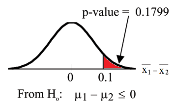
Calculate the p-value using the normal distribution: p-value = 0.1799
Graph:
425
Figure 10.2
x1 − x2 = 3 − 2.9 = 0.1
Compare α and the p-value: α = 0.05 and p-value = 0.1799. Therefore, α < p-value.
Make a decision: Since α < p-value, do not reject Ho.
Conclusion: At the 5% level of significance, from the sample data, there is not sufficient evidence
to conclude that the mean time wax 1 lasts is longer (wax 1 is more effective) than the mean time
wax 2 lasts.
NOTE: TI-83+ and TI-84: Press ❙❚❆❚. Arrow over to ❚❊❙❚❙ and press ✸✿✷✲❙❛♠♣❩❚❡st. Arrow over
to ❙t❛ts and press ❊◆❚❊❘. Arrow down and enter ✳✸✸ for sigma1, ✳✸✻ for sigma2, ✸ for the first
sample mean, ✷✵ for n1, ✷✳✾ for the second sample mean, and ✷✵ for n2. Arrow down to µ 1: and
arrow to > µ 2. Press ❊◆❚❊❘. Arrow down to ❈❛❧❝✉❧❛t❡ and press ❊◆❚❊❘. The p-value is p = 0.1799
and the test statistic is 0.9157. Do the procedure again but instead of ❈❛❧❝✉❧❛t❡ do ❉r❛✇.
10.4 Comparing Two Independent Population Proportions4
1. The two independent samples are simple random samples that are independent.
2. The number of successes is at least five and the number of failures is at least five for each of the
samples.
Comparing two proportions, like comparing two means, is common. If two estimated proportions are
different, it may be due to a difference in the populations or it may be due to chance. A hypothesis test can
help determine if a difference in the estimated proportions (PA − PB) reflects a difference in the population
proportions.
The difference of two proportions follows an approximate normal distribution. Generally, the null hypoth-
esis states that the two proportions are the same. That is, Ho : pA = pB. To conduct the test, we use a pooled
proportion, pc.
4This content is available online at <http://cnx.org/content/m17043/1.12/>.
CHAPTER 10. HYPOTHESIS TESTING: TWO MEANS, PAIRED DATA, TWO
426
PROPORTIONS
The pooled proportion is calculated as follows:
x
p
A + xB
c =
(10.7)
nA + nB
The distribution for the differences is:
1
1
P’A − P’B ∼ N 0,
pc · (1 − pc) ·
+
(10.8)
nA
nB
The test statistic (z-score) is:
(p’ − p’ ) − (p
z =
A
B
A − pB)
(10.9)
pc · (1 − pc) ·
1 + 1
nA
nB
Example 10.4: Two population proportions
Two types of medication for hives are being tested to determine if there is a difference in the
proportions of adult patient reactions. Twenty out of a random sample of 200 adults given med-
ication A still had hives 30 minutes after taking the medication. Twelve out of another random
sample of 200 adults given medication B still had hives 30 minutes after taking the medication.
Test at a 1% level of significance.
10.4.1 Determining the solution
This is a test of 2 population proportions.
Problem
(Solution on p. 456.)
How do you know?
Let A and B be the subscripts for medication A and medication B. Then pA and pB are the desired
population proportions.
Random Variable:
P’A − P’B = difference in the proportions of adult patients who did not react after 30 minutes to
medication A and medication B.
Ho : pA = pB
pA − pB = 0
Ha : pA = pB
pA − pB = 0
The words "is a difference" tell you the test is two-tailed.
Distribution for the test: Since this is a test of two binomial population proportions, the distribu-
tion is normal:
pc = xA+xB = 20+12 = 0.08
1 − p
n
c = 0.92
A +nB
200+200
Therefore,
P’A − P’B ∼ N 0,
(0.08) · (0.92) ·
1 + 1
200
200
P’A − P’B follows an approximate normal distribution.
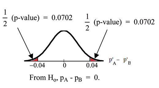
Calculate the p-value using the normal distribution: p-value = 0.1404.
427
Estimated proportion for group A:
p’ = xA = 20 =
A
0.1
nA
200
Estimated proportion for group B:
p’ = xB = 12 =
B
0.06
nB
200
Graph:
Figure 10.3
P’A − P’B = 0.1 − 0.06 = 0.04.
Half the p-value is below -0.04 and half is above 0.04.
Compare α and the p-value: α = 0.01 and the p-value = 0.1404. α < p-value.
Make a decision: Since α < p-value, do not reject Ho.
Conclusion: At a 1% level of significance, from the sample data, there is not sufficient evidence to
conclude that there is a difference in the proportions of adult patients who did not react after 30
minutes to medication A and medication B.
NOTE: TI-83+ and TI-84: Press ❙❚❆❚. Arrow over to ❚❊❙❚❙ and press ✻✿✷✲Pr♦♣❩❚❡st. Arrow down
and enter ✷✵ for x1, ✷✵✵ for n1, ✶✷ for x2, and ✷✵✵ for n2. Arrow down to ♣✶: and arrow to ♥♦t
❡q✉❛❧ ♣✷. Press ❊◆❚❊❘. Arrow down to ❈❛❧❝✉❧❛t❡ and press ❊◆❚❊❘. The p-value is p = 0.1404
and the test statistic is 1.47. Do the procedure again but instead of ❈❛❧❝✉❧❛t❡ do ❉r❛✇.
10.5 Matched or Paired Samples5
1. Simple random sampling is used.
2. Sample sizes are often small.
3. Two measurements (samples) are drawn from the same pair of individuals or objects.
4. Differences are calculated from the matched or paired samples.
5. The differences form the sample that is used for the hypothesis test.
5This content is available online at <http://cnx.org/content/m17033/1.15/>.
CHAPTER 10. HYPOTHESIS TESTING: TWO MEANS, PAIRED DATA, TWO
428
PROPORTIONS
6. The matched pairs have differences that either come from a population that is normal or the number of
differences is sufficiently large so the distribution of the sample mean of differences is approximately
normal.
In a hypothesis test for matched or paired samples, subjects are matched in pairs and differences are cal-
culated. The differences are the data. The population mean for the differences, µ d, is then tested using
a Student-t test for a single population mean with n − 1 degrees of freedom where n is the number of
diffe