11.1 The Chi-Square Distribution1
11.1.1 Student Learning Outcomes
By the end of this chapter, the student should be able to:
• Interpret the chi-square probability distribution as the sample size changes.
• Conduct and interpret chi-square goodness-of-fit hypothesis tests.
• Conduct and interpret chi-square test of independence hypothesis tests.
• Conduct and interpret chi-square homogeneity hypothesis tests.
• Conduct and interpret chi-square single variance hypothesis tests.
11.1.2 Introduction
Have you ever wondered if lottery numbers were evenly distributed or if some numbers occurred with a
greater frequency? How about if the types of movies people preferred were different across different age
groups? What about if a coffee machine was dispensing approximately the same amount of coffee each
time? You could answer these questions by conducting a hypothesis test.
You will now study a new distribution, one that is used to determine the answers to the above examples.
This distribution is called the Chi-square distribution.
In this chapter, you will learn the three major applications of the Chi-square distribution:
• The goodness-of-fit test, which determines if data fit a particular distribution, such as with the lottery
example
• The test of independence, which determines if events are independent, such as with the movie exam-
ple
• The test of a single variance, which tests variability, such as with the coffee example
NOTE: Though the Chi-square calculations depend on calculators or computers for most of the
calculations, there is a table available (see the Table of Contents 15. Tables). TI-83+ and TI-84
calculator instructions are included in the text.
1This content is available online at <http://cnx.org/content/m17048/1.9/>.
461
462
CHAPTER 11. THE CHI-SQUARE DISTRIBUTION
11.1.3 Optional Collaborative Classroom Activity
Look in the sports section of a newspaper or on the Internet for some sports data (baseball averages, bas-
ketball scores, golf tournament scores, football odds, swimming times, etc.). Plot a histogram and a boxplot
using your data. See if you can determine a probability distribution that your data fits. Have a discussion
with the class about your choice.
11.2 Notation2
The notation for the chi-square distribution is:
2
2
χ ∼ χ df
where d f = degrees of freedom depend on how chi-square is being used. (If you want to practice calculat-
ing chi-square probabilities then use d f = n − 1. The degrees of freedom for the three major uses are each
calculated differently.)
For the
2
χ
distribution, the population mean is µ = d f and the population standard deviation is σ =
2 · d f .
The random variable is shown as 2
χ but may be any upper case letter.
The random variable for a chi-square distribution with k degrees of freedom is the sum of k independent,
squared standard normal variables.
2
χ = (Z1)2 + (Z2)2 + ... + (Zk)2
11.3 Facts About the Chi-Square Distribution3
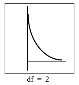
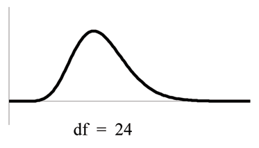
1. The curve is nonsymmetrical and skewed to the right.
2. There is a different chi-square curve for each d f .
2This content is available online at <http://cnx.org/content/m17052/1.6/>.
3This content is available online at <http://cnx.org/content/m17045/1.6/>.
463
(a)
(b)
Figure 11.1
3. The test statistic for any test is always greater than or equal to zero.
4. When d f > 90, the chi-square curve approximates the normal. For X ∼ 2
χ
the mean,
√
1000
µ = d f = 1000
and the standard deviation, σ =
2 · 1000 = 44.7. Therefore, X ∼ N (1000, 44.7), approximately.
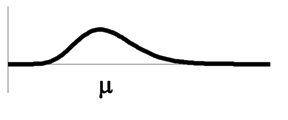
5. The mean, µ, is located just to the right of the peak.
Figure 11.2
In the next sections, you will learn about four different applications of the Chi-Square Distribution. These
hypothesis tests are almost always right-tailed tests. In order to understand why the tests are mostly right-
tailed, you will need to look carefully at the actual definition of the test statistic. Think about the following
while you study the next four sections. If the expected and observed values are "far" apart, then the test
statistic will be "large" and we will reject in the right tail. The only way to obtain a test statistic very close to
zero, would be if the observed and expected values are very, very close to each other. A left-tailed test could
be used to determine if the fit were "too good." A "too good" fit might occur if data had been manipulated
or invented. Think about the implications of right-tailed versus left-tailed hypothesis tests as you learn the
applications of the Chi-Square Distribution.
464
CHAPTER 11. THE CHI-SQUARE DISTRIBUTION
11.4 Goodness-of-Fit Test4
In this type of hypothesis test, you determine whether the data "fit" a particular distribution or not. For
example, you may suspect your unknown data fit a binomial distribution. You use a chi-square test (mean-
ing the distribution for the hypothesis test is chi-square) to determine if there is a fit or not. The null
and the alternate hypotheses for this test may be written in sentences or may be stated as equations or
inequalities.
The test statistic for a goodness-of-fit test is:
Σ (O − E)2
(11.1)
k
E
where:
• O = observed values (data)
• E = expected values (from theory)
• k = the number of different data cells or categories
The observed values are the data values and the expected values are the values you would expect to get
if the null hypothesis were true. There are n terms of the form (O−E)2 .
E
The degrees of freedom are df = (number of categories - 1).
The goodness-of-fit test is almost always right tailed. If the observed values and the corresponding ex-
pected values are not close to each other, then the test statistic can get very large and will be way out in the
right tail of the chi-square curve.
NOTE: The expected value for each cell needs to be at least 5 in order to use this test.
Example 11.1
Absenteeism of college students from math classes is a major concern to math instructors because
missing class appears to increase the drop rate. Suppose that a study was done to determine if the
actual student absenteeism follows faculty perception. The faculty expected that a group of 100
students would miss class according to the following chart.
Number absences per term
Expected number of students
0 - 2
50
3 - 5
30
6 - 8
12
9 - 11
6
12+
2
Table 11.1
A random survey across all mathematics courses was then done to determine the actual number
(observed) of absences in a course. The next chart displays the result of that survey.
4This content is available online at <http://cnx.org/content/m17192/1.8/>.
465
Number absences per term
Actual number of students
0 - 2
35
3 - 5
40
6 - 8
20
9 - 11
1
12+
4
Table 11.2
Determine the null and alternate hypotheses needed to conduct a goodness-of-fit test.
Ho: Student absenteeism fits faculty perception.
The alternate hypothesis is the opposite of the null hypothesis.
Ha: Student absenteeism does not fit faculty perception.
Problem 1
Can you use the information as it appears in the charts to conduct the goodness-of-fit test?
Solution
No. Notice that the expected number of absences for the "12+" entry is less than 5 (it is 2).
Combine that group with the "9 - 11" group to create new tables where the number of students for
each entry are at least 5. The new tables are below.
Number absences per term
Expected number of students
0 - 2
50
3 - 5
30
6 - 8
12
9+
8
Table 11.3
Number absences per term
Actual number of students
0 - 2
35
3 - 5
40
6 - 8
20
9+
5
Table 11.4
Problem 2
What are the degrees of freedom (d f )?
466
CHAPTER 11. THE CHI-SQUARE DISTRIBUTION
Solution
There are 4 "cells" or categories in each of the new tables.
d f = number o f cells − 1 = 4 − 1 = 3
Example 11.2
Employers particularly want to know which days of the week employees are absent in a five
day work week. Most employers would like to believe that employees are absent equally dur-
ing the week. Suppose a random sample of 60 managers were asked on which day of the week
did they have the highest number of employee absences. The results were distributed as fol-
lows:
Day of the Week Employees were most Absent
Monday
Tuesday
Wednesday
Thursday
Friday
Number of Absences
15
12
9
9
15
Table 11.5
Problem
For the population of employees, do the days for the highest number of absences occur with equal
frequencies during a five day work week? Test at a 5% significance level.
Solution
The null and alternate hypotheses are:
• Ho: The absent days occur with equal frequencies, that is, they fit a uniform distribution.
• Ha: The absent days occur with unequal frequencies, that is, they do not fit a uniform distri-
bution.
If the absent days occur with equal frequencies, then, out of 60 absent days (the total in the sample:
15 + 12 + 9 + 9 + 15 = 60), there would be 12 absences on Monday, 12 on Tuesday, 12 on Wednesday,
12 on Thursday, and 12 on Friday. These numbers are the expected (E) values. The values in the
table are the observed (O) values or data.
This time, calculate the 2
χ test statistic by hand. Make a chart with the following headings and fill
in the columns:
• Expected (E) values (12, 12, 12, 12, 12)
• Observed (O) values (15, 12, 9, 9, 15)
• (O − E)
• (O − E)2
• (O − E)2
E
The last column ( (O − E)2 ) should have 0.75, 0, 0.75, 0.75, 0.75.
E
Now add (sum) the last column. Verify that the sum is 3. This is the 2
χ test statistic.
To find the p-value, calculate P
2
χ > 3 . This test is right-tailed.
(Use a computer or calculator to find the p-value. You should get p-value = 0.5578.)
467
The d f s are the number of cells − 1 = 5 − 1 = 4.
TI-83+ and TI-84: Press ✷♥❞ ❉■❙❚❘. Arrow down to 2
χ ❝❞❢. Press ❊◆❚❊❘. Enter ✭✸✱✶✵❫✾✾✱✹✮.
Rounded to 4 decimal places, you should see 0.5578 which is the p-value.
Next, complete a graph like the one below with the proper labeling and shading. (You should
shade the right tail.)
The decision is to not reject the null hypothesis.
Conclusion: At a 5% level of significance, from the sample data, there is not sufficient evidence to
conclude that the absent days do not occur with equal frequencies.
NOTE: TI-83+ and some TI-84 calculators do not have a special program for the test statistic for the
goodness-of-fit test. The next example (Example 11-3) has the calculator instructions. The newer
TI-84 calculators have in ❙❚❆❚ ❚❊❙❚❙ the test ❈❤✐✷ ●❖❋. To run the test, put the observed values
(the data) into a first list and the expected values (the values you expect if the null hypothesis is
true) into a second list. Press ❙❚❆❚ ❚❊❙❚❙ and ❈❤✐✷ ●❖❋. Enter the list names for the Observed list
and the Expected list. Enter the degrees of freedom and press ❝❛❧❝✉❧❛t❡ or ❞r❛✇. Make sure you
clear any lists before you start. See below.
NOTE: To Clear Lists in the calculators: Go into ❙❚❆❚ ❊❉■❚ and arrow up to the list name area of
the particular list. Press ❈▲❊❆❘ and then arrow down. The list will be cleared. Or, you can press
❙❚❆❚ and press 4 (for ❈❧r▲✐st). Enter the list name and press ❊◆❚❊❘.
Example 11.3
One study indicates that the number of televisions that American families have is distributed (this
is the given distribution for the American population) as follows:
Number of Televisions
Percent
0
10
1
16
2
55
3
11
over 3
8
Table 11.6
468
CHAPTER 11. THE CHI-SQUARE DISTRIBUTION
The table contains expected (E) percents.
A random sample of 600 families in the far western United States resulted in the following data:
Number of Televisions
Frequency
0
66
1
119
2
340
3
60
over 3
15
Total = 600
Table 11.7
The table contains observed (O) frequency values.
Problem
At the 1% significance level, does it appear that the distribution "number of televisions" of far
western United States families is different from the distribution for the American population as a
whole?
Solution
This problem asks you to test whether the far western United States families distribution fits the
distribution of the American families. This test is always right-tailed.
The first table contains expected percentages. To get expected (E) frequencies, multiply the per-
centage by 600. The expected frequencies are:
Number of Televisions
Percent
Expected Frequency
0
10
(0.10) · (600) = 60
1
16
(0.16) · (600) = 96
2
55
(0.55) · (600) = 330
3
11
(0.11) · (600) = 66
over 3
8
(0.08) · (600) = 48
Table 11.8
Therefore, the expected frequencies are 60, 96, 330, 66, and 48. In the TI calculators, you can let the
calculator do the math. For example, instead of 60, enter .10*600.
Ho: The "number of televisions" distribution of far western United States families is the same as
the "number of televisions" distribution of the American population.
Ha: The "number of televisions" distribution of far western United States families is different from
the "number of televisions" distribution of the American population.
Distribution for the test: 2
χ where d f = (the number of cells) − 1 = 5 − 1 = 4.
4
NOTE: d f = 600 − 1
469
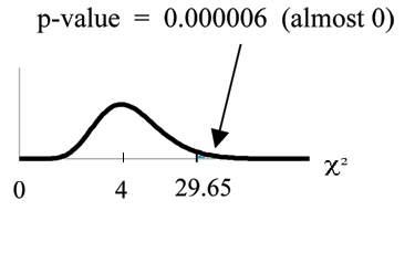
Calculate the test statistic: 2
χ = 29.65
Graph:
Probability statement: p-value = P
2
χ > 29.65
= 0.000006.
Compare α and the p-value:
• α = 0.01
• p-value = 0.000006
So, α > p-value.
Make a decision: Since α > p-value, reject Ho.
This means you reject the belief that the distribution for the far western states is the same as that
of the American population as a whole.
Conclusion: At the 1% significance level, from the data, there is sufficient evidence to conclude
that the "number of televisions" distribution for the far western United States is different from the
"number of televisions" distribution for the American population as a whole.
NOTE: TI-83+ and some TI-84 calculators: Press ❙❚❆❚ and ❊◆❚❊❘. Make sure to clear lists ▲✶,
▲✷, and ▲✸ if they have data in them (see the note at the end of Example 11-2). Into ▲✶, put
the observed frequencies ✻✻, ✶✶✾, ✸✹✾, ✻✵, ✶✺. Into ▲✷, put the expected frequencies ✳✶✵✯✻✵✵✱
✳✶✻✯✻✵✵, ✳✺✺✯✻✵✵, ✳✶✶✯✻✵✵, ✳✵✽✯✻✵✵. Arrow over to list ▲✸ and up to the name area ✧▲✸✧. Enter
✭▲✶✲▲✷✮❫✷✴▲✷ and ❊◆❚❊❘. Press ✷♥❞ ◗❯■❚. Press ✷♥❞ ▲■❙❚ and arrow over to ▼❆❚❍. Press ✺. You
should see ✧s✉♠✧ ✭❊♥t❡r ▲✸✮. Rounded to 2 decimal places, you should see ✷✾✳✻✺. Press ✷♥❞
❉■❙❚❘. Press ✼ or Arrow down to ✼✿ χ✷❝❞❢ and press ❊◆❚❊❘. Enter ✭✷✾✳✻✺✱✶❊✾✾✱✹✮. Rounded
to 4 places, you should see ✺✳✼✼❊✲✻ ❂ ✳✵✵✵✵✵✻ (rounded to 6 decimal places) which is the p-value.
The newer TI-84 calculators have in ❙❚❆❚ ❚❊❙❚❙ the test ❈❤✐✷ ●❖❋. To run the test, put the
observed values (the data) into a first list and the expected values (the values you expect if the
null hypothesis is true) into a second list. Press ❙❚❆❚ ❚❊❙❚❙ and ❈❤✐✷ ●❖❋. Enter the list names
for the Observed list and the Expected list. Enter the degrees of freedom and press ❝❛❧❝✉❧❛t❡ or
❞r❛✇. Make sure you clear any lists before you start.
Example 11.4
Suppose you flip two coins 100 times. The results are 20 HH, 27 HT, 30 TH, and 23 TT. Are the
coins fair? Test at a 5% significance level.
470
CHAPTER 11. THE CHI-SQUARE DISTRIBUTION
Solution
This problem can be set up as a goodness-of-fit problem. The sample space for flipping two fair
coins is {HH, HT, TH, TT}. Out of 100 flips, you would expect 25 HH, 25 HT, 25 TH, and 25 TT.
This is the expected distribution. The question, "Are the coins fair?" is the same as saying, "Does
the distribution of the coins (20 HH, 27 HT, 30 TH, 23 TT) fit the expected distribution?"
Random Variable: Let X = the number of heads in one flip of the two coins. X takes on the value
0, 1, 2. (There are 0, 1, or 2 heads in the flip of 2 coins.) Therefore, the number of cells is 3. Since
X = the number of heads, the observed frequencies are 20 (for 2 heads), 57 (for 1 head), and 23 (for
0 heads or both tails). The expected frequencies are 25 (for 2 heads), 50 (for 1 head), and 25 (for 0
heads or both tails). This test is right-tailed.
Ho: The coins are fair.
Ha: The coins are not fair.
Distribution for the test: 2
χ 2 where d f = 3 − 1 = 2.
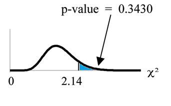
Calculate the test statistic: 2
χ = 2.14
Graph:
Probability statement: p-value = P
2
χ > 2.14
= 0.3430
Compare α and the p-value:
• α = 0.05
• p-value = 0.3430
So, α < p-value.
Make a decision: Since α < p-value, do not reject Ho.
Conclusion: There is insufficient evidence to conclude that the coins are not fair.
NOTE: TI-83+ and some TI- 84 calculators: Press ❙❚❆❚ and ❊◆❚❊❘. Make sure you clear lists ▲✶, ▲✷,
and ▲✸ if they have data in them. Into ▲✶, put the observed frequencies ✷✵, ✺✼, ✷✸. Into ▲✷, put
the expected frequencies ✷✺, ✺✵, ✷✺. Arrow over to list ▲✸ and up to the name area ✧▲✸✧. Enter
✭▲✶✲▲✷✮❫✷✴▲✷ and ❊◆❚❊❘. Press ✷♥❞ ◗❯■❚. Press ✷♥❞ ▲■❙❚ and arrow over to ▼❆❚❍. Press ✺. You
should see ✧s✉♠✧.❊♥t❡r ▲✸. Rounded to 2 decimal places, you should see ✷✳✶✹. Press ✷♥❞ ❉■❙❚❘.
Arrow down to ✼✿ χ✷❝❞❢ (or press ✼). Press ❊◆❚❊❘. Enter ✷✳✶✹✱✶❊✾✾✱✷✮. Rounded to 4 places, you
should see ✳✸✹✸✵ which is the p-value.
The newer TI-84 calculators have in ❙❚❆❚ ❚❊❙❚❙ the test ❈❤✐✷ ●❖❋. To run the test, put the
471
observed values (the data) into a first list and the expected values (the values you expect if the
null hypothesis is true) into a second list. Press ❙❚❆❚ ❚❊❙❚❙ and ❈❤✐✷ ●❖❋. Enter the list names
for the Observed list and the Expected list. Enter the degrees of freedom and press ❝❛❧❝✉❧❛t❡ or
❞r❛✇. Make sure you clear any lists before you start.
11.5 Test of Independence5
Tests of independence involve using a contingency table of observed (data) values. You first saw a contin-
gency table when you studied probability in the Probability Topics (Section 4.1) chapter.
The test statistic for a test of independence is similar to that of a goodness-of-fit test:
Σ (O − E)2
(11.2)
(i·j)
E
where:
• O = observed values
• E = expected values
• i = the number of rows in the table
• j = the number of columns in the table
There are i · j terms of the form (O−E)2 .
E
A test of independence determines whether two factors are independent or not. You first e