Discrete Time Systems
On the other side, one sees that small differences of η −η
r
or equivalently small values
tn
rtn+ 1
η
−η
r
r
of ˙ η
|
− tn+ 1
tn
r
have the influence of decreasing |f as well. Since the quantity ˙ η
assumes
tn
1
rtn
h
small values for h small, then large cruise velocities do not affect the performance if the
sampling time is chosen relatively small.
Besides, the term hJt v in f leads to the same conclusion about the effect of h. However,
n
tn
1
it is interesting to stress the fact that appears in vehicle rotations which may rise the norm
of Jt [ ϕ, θ, ψ] considerably when the pitch angle goes above about 30 ◦ (Jordán & Bustamante,
n
2011).
The scalar function f 4, whose bound is implicitly included in (78) gets small when particularly
the vector b is small (this means also τn small), and the motion vector function s is also
2
tn
rather moderate.
Finally, there is the term 2hτ2 in (74) that also contributes to increase f
particularly when
n
Δ Q 2 n
saturation values of the thrusters are achieved. Since τ2 is fixed by the controller, the only
n
countermeasure to be applied lays in the fact that the controller always choose the lower τ2n
of the two possible roots in (46). So, the perturbation energy fΔ Q is reduced as far as possible
2 n
by the controller.
From (63) one can draw out that the choice Kv = 1 M
h
b in the negative definite terms is much
∗
more appropriate to increase the negativeness of Δ Qt . Equally the choice of Kp in the same
n
manner helps the trajectories to get the residual set more rapid.
Besides,
the
model
errors
and
noisy
measures
( εv + δv
−δv
)
and
n+ 1
tn+ 1
tn+ 1
εη + δη
−δv t
enter linearly and quadratically in the energy equation (74).
As
n+ 1
tn+ 1
n+ 1
they are usually small, only the linear terms are magnified/attenuated by f , f , f and τ ,
1
2
3
2n
while f 4 impacts nonlinearly in τn and s as seen in (54).
2
tn
5.5 Instability for large sampling time
Broadly speaking, the influence of the analyzed parameters will play a role in the instability
when (on the chosen h is something large, even smaller than one, because the quadratic terms
rise significantly to turn to be dominant in the error function f ∗
Δ Q .
n
∗
The study of this phenomenon is rather complex but it generally involves the function Δ Qtn
in (63) and f ∗
Δ Q in (64).
n
For instante, when
T
T
∗
∗
f ∗
Δ
> η
+
Q
hKp hKp − 2 I η
v hK
,
(81)
n
tn
tn
tn
v
hKv − 2 I v tn
the path trajectories may not be bounded into a residual set because the domain for the
initial conditions in this situation is partially repulsive. So, depending on the particular initial
conditions and for h >> 0 the adaptive control system may turn unstable.
In conclusion, when comparing two digital controllers, the sensitivity of the stability to h is
fundamental to draw out robust properties and finally to range them.
6. Adaptive control algorithm
The adaptive control algorithm can be summarized as follows.
Preliminaries:
1) Estimate a lower bound M , for instance M = Mb (Jordán & Bustamante, 2011),
A General Approach to Discrete-Time Adaptive Control Systems with Perturbed Measures for
Complex Dynamics - Case Study: Unmanned Underwater Vehicles
273
2) Select a sampling time h as smaller as possible
3) Choose design gain matrices Kp and Kv according to (68)-(69), and simultaneously in order
∗
to reduce f ∗
Δ Q and Δ Q (see related commentary in previous section),
n
tn
4) Define the adaptive gain matrices Γ i (usually Γ i = αi I with αi > 0),
5) Stipulate the desired sampled-data path references for the geometric and kinematic
trajectories in 6 DOFś: ηr and v r , respectively (see related commentary in previous section).
tn
tn
Continuously at each sample point:
6) Calculate the control thrust τn with components τ1 in (30) and τ
(46) (or (72)),
n
2n
respectively,
7) Calculate the adaptive controller matrices (56) with the lower bound M instead of M.
Long-term tuning:
7) Redefine Kp, Kv and h in order to achieve optimal tracking performance.
7. Case study
7.1 Setup
With the end of illustrating the features of our control system approach, we simulate a
path-tracking problem in 6 DOFś for an underwater vehicle in a planar motion with some
sporadic immersions to the floor.
A continuous-time model of a fully-maneuverable underwater vehicle is employed for the
numerical simulations. Details of this dynamics are given in (Jordán & Bustamante, 2009c).
The propulsion system is composed by 8 thrusters, distributed in 4 vertical and 4 horizontal.
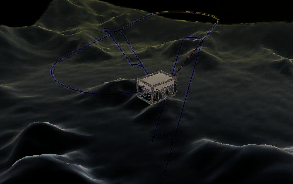
The simulated reference path ηr and the navigation path η are reproduced together by means
of a visualization program (see a photogram in Fig. 2). The units for the path run away are in
meters.
Basically the vehicle turns around a planar path. At a certain coordinate A it leaves the plane
and submerses to the point A for picking up a sample (of weight 10 (Kgf)) on the sea floor
and returns back to A with a typical maneuver (backward movement and rotation). Then it
continues on the planar trajectory till the coordinate B in where it submerses again to the point
B in order to place an equipment on the floor (of weight 20 (Kgf)) before to retreat and turn
back to B and to complete finally the cycle. The vehicle weight is about 60 (kgf).
Additionally to the geometric path, the rate function v r( t) = J− 1( η ) ·η (
r
r t) along it, is also
specified, with short periods of rest at points A and B before beginning and after ending the
maneuvers on the bottom.
At the start point of the mission (represented by O in Fig. 2), it is assumed for the adaptive
control there is no information available about the vehicle dynamics matrices. Moreover, the
maneuvers at stretches A- A and B- B imply considerable changes of moments acting on the
vehicle in both a positive and negative quantities.
The reference velocity is programmed to be constant equal to 0.25(m/s) for the advance and
as well as for the descent/ascent along the path. This rate will be referred to as the cruise
velocity.
By the simulations, the adaptive control algorithm summarized in the previous section, is
implemented. It is coupled with the ODE (1)-(2) for the vehicle dynamics, whose solution is
numerically calculated in continuous time using Runge-Kutta approximators (the so-called
ODE45). The computed control action is connected to a zero-order sample&hold previously
to excite the vehicle.
274
Discrete Time Systems
A
B
20(m)
O
5(m)
A’
ΔΜ > 0
10(m)
B’
ΔΜ < 0
Fig. 2. Path tracking with grab sampling at coordinate A , and with placing of an equipment
on the seafloor at coordinate B
7.2 Design parameters
The most important a-priori information for the adaptive controller design is the
ODE-structure in (1)-(2) but not its dynamics matrices, with the exception of the lower bound
for the inertia matrix M. This takes the form
M = Mb + Ma
(82)
with the components: the body matrix Mb and the additive matrix Ma given by
Mb = Mb + δ( t − t
n
A ) MbΔ+ − δ( t − tB ) MbΔ −
(83)
Ma = Ma + δ( t − t
n
A ) MaΔ+ − δ( t − tB ) MaΔ − ,
(84)
where Mb and M
are nominal values of M
n
an
b and Ma at the start point O, and
MbΔ −, MbΔ+, MaΔ+ and MaΔ − are positive and negative variations at instants tA and tB on the points A and B of Fig. 2. Here δ( t − ti) represents the Dirac function.
For our application Mb is determinable beforehand experimentally and it is set as the lower
n
bound M for the control and adaptive laws. In the simulated scenario, MbΔ − is assumed
known because it is about of an equipment deposited on the seafloor. In the case of MbΔ+,
MaΔ+ and even MaΔ −, we depart from unknown values.
The property of Ma ≥ 0 is not affected by the sign of MaΔ+ and MaΔ −, which may be positive
and negative as well. For that reason, a valid lower bound is chosen as M = Mb − M
n
bΔ − .
Taking into account the simulation setup for the weight changes (the weight picked up from
the seafloor at tA and the second weight deposited on the seafloor at tB ), the lower bound for
M is
M = diag(60, 60, 60, 5, 10, 10),
(85)
A General Approach to Discrete-Time Adaptive Control Systems with Perturbed Measures for
Complex Dynamics - Case Study: Unmanned Underwater Vehicles
275
and the mass variations are
MbΔ+ = diag(10, 10, 10, 0.6250, 4.2250, 3.6)
(86)
MbΔ − = diag(20, 20, 20, 1.25, 1.25, 0)
(87)
MaΔ+ = diag(6.3, 15.4, 0.115, 0.115, 0.261, 0.276)
(88)
MaΔ − = diag(12.6, 30.8, 0.23, 0.23, 0.521, 0.551).
(89)
The design gain matrices for the controller are
Kp = diag (5, 5, 5, 5, 5, 5)
Kv = diag (300, 300, 300, 25, 50, 50)
(90)
and the adaptive gain matrices about
Γ i = I.
(91)
Finally we have proposed a sampling time h = 0.2(s).
All quantities are expressed in the SI Units.
7.3 Control performance
Here the acquired performance by the autonomously guided vehicle under the described
simulated setup will be evaluated. First, in Fig. 3, the path error evolution corresponding
to every mode with their respective rates is shown for the different transient phases, namely:
the controller autotuning at the initial phase (to the left), the sampling phase on the sea bottom
at A (in the middle), and the release of an equipment on the floor at B (to the right).
The largest path errors had occurred during the initial phase because the amount of
information for the control adaptation was null. Here, the longest transient took about 5(s)
which is considered outstanding in comparison to the commonly slow open loop behavior.
Later, after the mass changes, the path errors behaved much more moderate and were
insignificant in magnitude (only a few centimeters or a few hundredths of a radian according
to translation/rotation). Among them, the errors in the surge, sway and pitch modes ( x, z and
θ) resulted more perturbed than the remainder ones because they were more excited from the
main motion provided by the stipulated mission. In all evolutions the adaptations occurred
quick and smoothly.
The same scenario of control performance can be observed in Fig. 4 from the side of the
velocity path errors for every mode of motion. Qualitatively, all kinematic path errors were
attenuated rapid and smoothly in the autotuning phase as well as during the mass-change
periods. The magnitude of these errors is also related to the rapid changes of the reference v ref
in the programmed maneuvers.
In the Fig. 5, the time evolution of the actuator thrust for two arbitrarily selected thrusters
(one horizontal and one vertical) is shown. Analogously as previous results, the forces are
compared within the three periods of transients. One observes that the intervention of the
controller after a sudden change of mass occurred immediately. Also the transients of these
interventions up to the practical steady state were relatively short.
Fig. 6 illustrates the time evolution of some controller matrices Ui. To this end, we had chosen
the induced norm of U 8 which is partially related to the adaptation of the linear damping.
One sees that the norm of U 8 evolved with significative changes. In contrast to analog
adaptive controllers of the speed-gradient class, here the Ui’s do not tend asymptotically to
276
Discrete Time Systems
0.01
0.02
) 0.1
m
0
0.01
0.05
a x(
0
-0.01
0
tA’
tB’
-0.05
-0.02
-0.01
x 10-4
x 10-4
5
5
0.1
)
0
0
m 0.05
a y(
-5
-5
0
t
t
A’
B’
-0.05
-10
-10
0.01
0.01
0.1
)m 0.05
0
0
a z(
0
tA’
tB’
-0.05
-0.02
-0.02
x 10-3
x 10-3
5
5
0.2
0
0.1
0
(rad)
t
a
-5
0
ϕ
A’
tB’
-5
-10
x 10-3
0.01
10
0.2
0
ad)
0
0.1
(r
-0.01
tA’
a
-0.02
0
θ
t
-5
B’
x 10-3
x 10-3
)
5
5
0.2
d
0
0
0.1
(ra
a
-5
-5
t
0
ψ
tA’
B’
-10
-10
0
1
2
3
4
5
400
420
440
460
480
500
1020 1040 1060 1080 1100
time (s)
time (s)
time (s)
Fig. 3. Position path errors during transients in three different periods (from left to right
column: autotuning, adaptation by weight pick up and adaptation by weight deposit)
− 1
− 1
constant matrices because of the difference between M
and M
in (58)-(59) (cf. Jordán &
Bustamante, 2009c).
8. Conclusions
In this paper a novel design of adaptive control systems was presented. This is based on
speed-gradient techniques which are widespread in the form of continuous-time designs
in the literature. Here, we had focused their counterparts namely sampled-data adaptive
controllers.
The work was framed into the path tracking control problem for the guidance of vehicles
in many degrees of freedom.
Particularly, the most complex dynamics of this class
A General Approach to Discrete-Time Adaptive Control Systems with Perturbed Measures for
Complex Dynamics - Case Study: Unmanned Underwater Vehicles
277
)
0.2
0.1
/s
0
0
m
0
-0.2
-0.1
∼ u (
tA’
tB’
-0.4
-0.2
-0.2
x 10 -3
x 10 -3
5
2
0
0