When you began to study mathematics years ago, you began with basic arithmetic in the form of understanding numbers and basic operations. Later, as your basic understanding of mathematics grew, it began to divide itself into 'pure' mathematics and 'applied' mathematics. You will note, however, that what you began with, namely arithmetic, is largely 'pure': the use of numbers to represent quantities is, in fact, very abstract, and it is only after understanding how numbers relate to quantities that you can do 'applied' mathematics by considering how arithmetic relates to 'real world' situations. For instance, taking two piles of blocks and putting them together to get a total is equivalent to taking the individual quantities and summing them together.
Just as 'mathematics' can be divided into 'pure mathematics' (i.e. theory) and 'applied mathematics' (i.e. applications), so 'statistics' can be divided into 'probability theory' and 'applied statistics'. And just as you cannot do applied mathematics without knowing any theory, you cannot do statistics without beginning with some understanding of probability theory. Furthermore, just as it is not possible to describe what arithmetic is without describing what mathematics as a whole is, it is not possible to describe what probability theory is without some understanding of what statistics as a whole is about, and in its broadest sense, it is about 'processes'.
A process is the manner in which an object changes over time. This description is, of course, both very general and very abstract, so let's look at a common example. Consider a coin. Now, the coin by itself is not a process; it is simply an object. However, if I was to put the coin through a process by picking it up and flipping it in the air, after a certain amount of time (however long it would take to land), it is brought to a final state. We usually refer to this final state as 'heads' or 'tails' based on which side of the coin landed face up, and it is the 'heads' or 'tails' that the statistician is interested in. Without the process, however (i.e the object moving through time during the coin flip), there is nothing to analyze. Of course, leaving the coin stationary is also a process, but we already know that its final state is going to be the same as its original state, so it is not a particularly interesting process. Usually when we speak of a process, we mean one where the outcome is not yet known, otherwise there is no real point in analyzing it. With this understanding, it is very easy to understand what, precisely, probability theory is.
When we speak of probability theory as a whole, we mean the means and methods by which we quantify the possible outcomes of processes. Then, just as 'applied' mathematics takes the methods of 'pure' mathematics and applies them to real-world situations, applied statistics takes the means and methods of probability theory (i.e. the means and methods used to quantify possible outcomes of events) and applies them to real-world events in some way or another. For example, we might use probability theory to quantify the possible outcomes of the coin-flip above as having a 50% chance of coming up heads and a 50% chance of coming up tails, and then use statistics to apply it a real-world situation by saying that of six coins sitting on a table, the most likely scenario is that three coins will come up heads and three coins will come up tails. This, of course, may not happen, but if we were only able to bet on ONE outcome, we would probably bet on that because it is the most probable. But here, we are already getting ahead of ourselves. So let's back up a little.
To quantify results, we may use a variety of methods, terms, and notations, but a few common ones are:
a percentage (for example '50%')
a proportion of the total number of outcomes (for example, '5/10')
a proportion of 1 (for example, '1/2')
You may notice that all three of the above examples represent the same probability, and in fact ANY method of probability is fundamentally based on the following procedure:
Define a process.
Define the total measure for all outcomes of the process.
Describe the likelihood of each possible outcome of the process with respect to the total measure.
The term 'measure' may be confusing, but one may think of it as a ruler. If we take a metrestick, then half of that metrestick is 50 centimetres, a quarter of that metrestick is 25 centimetres, etc. However, the thing to remember is that without the metrestick, it makes no sense to talk about proportions of a metrestick! Indeed, the three examples above (50%, 5/10, and 1/2) represented the same probability, the only difference was how the total measure (ruler) was defined. If we go back to thinking about it in terms of a metrestick '50%' means '50/100', so it means we are using 50 parts of the original 100 parts (centimetres) to quantify the outcome in question. '5/10' means 5 parts out of the original 10 parts (10 centimetre pieces) depict the outcome in question. And in the last example, '1/2' means we are dividing the metrestick into two pieces and saying that one of those two pieces represents the outcome in question. But these are all simply different ways to talk about the same 50 centimetres of the original 100 centimetres! In terms of probability theory, we are only interested in proportions of a whole.
Although there are many ways to define a 'measure', the most common and easiest one to generalize is to use '1' as the total measure. So if we consider the coin-flip, we would say that (assuming the coin was fair) the likelihood of heads is 1/2 (i.e. half of one) and the likelihood of tails is 1/2. On the other hand, if we consider the event of not flipping the coin, then (assuming the coin was originally heads-side-up) the likelihood of heads is now 1, while the likelihood of tails is 0. But we could have also used '14' as the original measure and said that the likelihood of heads or tails on the coin-flip was each '7 out of 14', while on the non-coin-flip the likelihood of heads was '14 out of 14', and the likelihood of tails was '0 out of 14'. Similarly, if we consider the throwing of a (fair) six-sided die, it may be easiest to set the total measure to '6' and say that the likelihood of throwing a '4' is '1 out of the 6', but usually we simply say that it is 1/6.
The term random experiment or statistical experiment is used to describe any repeatable process, the results of which are analyzed in some way. For example, flipping a coin and noting whether or not it lands heads-up is a random experiment because the process is repeatable. On the other hand, your reading this sentence for the first time and noting whether you understand it is not a random experiment because it is not repeatable (though making a number of random people read it and noting which ones understand it would turn it into a random experiment).
There are three important concepts associated with a random experiment: 'outcome', 'sample space', and 'event'. Two examples of experiments will be used to familiarize you with these terms:
In Experiment 1 a single die is thrown and the value of the top face after it has come to rest is noted.
In Experiment 2 two dice are thrown at the same time and the total of the values of each of the top faces after they have come to rest is noted.
An outcome of an experiment is a single result of that experiment.
A possible outcome of Experiment 1: the value on the top face is '3'
A possible outcome of Experiment 2: the total value on the top faces is '9'
The sample space of an experiment is the complete set of possible outcomes of the experiment.
Experiment 1: the sample space is 1,2,3,4,5,6
Experiment 2: the sample space is 2,3,4,5,6,7,8,9,10,11,12
An event is any set of outcomes of an experiment. (You can think of it as 'the outcomes we are looking for' or favourable outcomes.)
A possible event of Experiment 1: an even number being on the top face of the die
A possible event of Experiment 2: the numbers on the top face of each die being equal
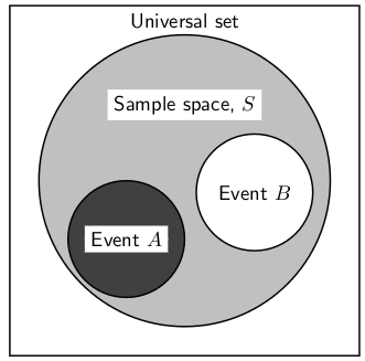
A Venn diagram can be used to show the relationship between the possible outcomes of a random experiment and the sample space. The Venn diagram in Figure 11.1 shows the difference between the universal set, a sample space and events and outcomes as subsets of the sample space.
Figure 11.1.
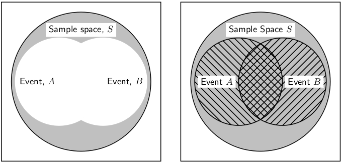
Venn diagrams can also be used to indicate the union and intersection between events in a sample space (Figure 11.2).
Figure 11.2.
Exercise 11.1.1. Random Experiments (Go to Solution)
In a box there are pieces of paper with the numbers from 1 to 9 written on them. A piece of paper is drawn from the box and the number on it is noted. Let S denote the sample space, let P denote the event 'drawing a prime number', and let E denote the event 'drawing an even number'. Using appropriate notation, in how many ways is it possible to draw: i) any number? ii) a prime number? iii) an even number? iv) a number that is either prime or even? v) a number that is both prime and even?
A final notion that is important to understand is the notion of complement. Just as in geometry when two angles were called 'complementary' if they added up to 180 degrees, (the two angles 'complement' each other to make a 'whole' straight line), the complement of a set of outcomes S , usually denoted S c is the set of all outcomes in the sample space but not in S (i.e., S c complements S to form the entire sample space). Thus, by definition, S∪S c = S is always true. So in the Exercise above, the complement of P (i.e. P^c) = {1,4,6,8,9}, while E^c = {1,3,5,7,9}. So n(P^c) = n(E^c) = 5
In theory, it is very easy to calculate complements, since the number of elements in the complement of a set is just the total number of outcomes in the sample space minus the outcomes in that set (in the example above, there were 9 possible outcomes in the sample space, and 4 possible outcomes in each of the sets we were interested in, thus both complements contained 9-4 = 5 elements). Similarly, it is easy to calculate probabilities of complements of events since they are simply the total probability (e.g. 1 if our total measure is 1) minus the probability of the event in question.
Let S denote the set of whole numbers from 1 to 16, X denote the set of even numbers from 1 to 16 and Y denote the set of prime numbers from 1 to 16
Draw a Venn diagram accurately depicting S , X and Y .
Find n(S), n(X), n(Y), n(X∪Y), n(X∩Y).
There are 79 Grade 10 learners at school. All of these take either Maths, Geography or History. The number who take Geography is 41, those who take History is 36, and 30 take Maths. The number who take Maths and History is 16; the number who take Geography and History is 6, and there are 8 who take Maths only and 16 who take only History.
Draw a Venn diagram to illustrate all this information.
How many learners take Maths and Geography but not History?
How many learners take Geography only?
How many learners take all three subjects?
Pieces of paper labelled with the numbers 1 to 12 are placed in a box and the box is shaken. One piece of paper is taken out and then replaced.
What is the sample space, S ?
Write down the set A , representing the event of taking a piece of paper labelled with a factor of 12.
Write down the set B , representing the event of taking a piece of paper labelled with a prime number.
Represent A , B and S by means of a Venn diagram.
Find
n(S)
n(A)
n(B)
n(A∩B)
n(A∪B)
Is n(A∪B) = n(A) + n(B) – n(A∩B)?
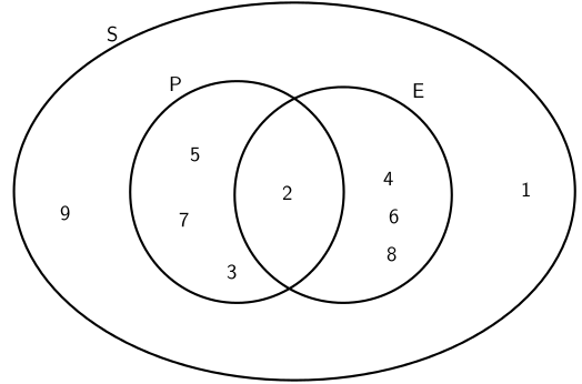
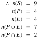
Solution to Exercise 11.1.1. (Return to Exercise)
Consider the events: :
Drawing a prime number: P = {2;3;5;7}
Drawing an even number: E = {2;4;6;8}
Figure 11.3.
The union of
P
and
E
is the set of all elements in
P
or in
E
(or in both). 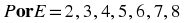 .
.  is also written
P∪E
.
is also written
P∪E
.
The intersection of
P
and
E
is the set of all elements in both
P
and
E
.  .
.  is also written as
P∩E
.
is also written as
P∩E
.
We use n(S) to refer to the number of elements in a set S , n(X) for the number of elements in X , etc.
Probability is connected with uncertainty. In any statistical experiment, the outcomes that occur may be known, but exactly which one might occur is usually not known. Mathematically, probability theory formulates incomplete knowledge pertaining to the likelihood of an occurrence. For example, a meteorologist might say there is a 60% chance that it will rain tomorrow. This means that in 6 of every 10 times when the world is in the current state, it will rain tomorrow.
In everyday speech, we often refer to probabilities using percentages between 0% and 100%. A probability of 100% (100 out of 100) means that an event is certain, whereas a probability of 0% (0 out of 100) is often taken to mean the event is impossible. However, in certain circumstances, there can be a distinction between logically impossible and occurring with zero probability if the sample space is large enough (i.e. infinite) or in some other way indeterminate. For example, in selecting a random fraction between 0 and 1, the probability of selecting 1/2 is 0, but it is not logically impossible (since there are infinitely many numbers), while trying to predict the exact number of raindrops to fall into a large enough area is also 0 (or close to it), since the possible number of raindrops that might occur at a given time is both very large and difficult to determine.
Another way of referring to probabilities is odds. The odds of an event is defined as the ratio of the probability that the event occurs to the probability that it does not occur. For example, the odds of a coin landing on a given side are  , usually written "1 to 1" or "1:1". This means that on average, the coin will land on that side as many times as it will land on the other side.
We say two outcomes are equally likely if they have an equal chance of happening. For example when a fair coin is tossed, each outcome in the sample space S = {h