ei(k −k)xu∗k,n(x)uk ,m(x)dx,
p
−a/2
where the sum over p runs over all the N vectors of the lattice. The purely
geometric factor multiplying the integral differs from zero only if k and k
coincide:
eip(k −k)a = N δk,k .
(9.9)
p
we have used Kronecker’s delta, not Dirac’s delta, because the k form a dense
but still finite set (there are N of them). We note that the latter orthogonality
relation holds for whatever periodic part, u(x), the Bloch states may have.
Nothing implies that the periodic parts of the Bloch states at different k are
orthogonal: only those for different Bloch states at the same k are orthogonal
(see Eq.(9.7)).
9.1.5
Plane-wave basis set
Let us come back to the numerical solution. We look for the solution using a
plane-wave basis set. This is especially appropriate for problems in which the
potential is periodic. We cannot choose any plane-wave set, though: the correct
choice is restricted by the Bloch vector and by the periodicity of the system.
Given the Bloch vector k, the “right” plane-wave basis set is the following:
1
2π
bn,k(x) = √ ei(k+Gn)x,
Gn =
n.
(9.10)
L
a
The “right” basis must in fact have a exp(ikx) behavior, like the Bloch states
with Bloch vector k; moreover the potential must have nonzero matrix elements
between plane waves. For a periodic potential like the one in Eq.(9.4), matrix elements:
1
L/2
bi,k|V |bj,k
=
V (x)e−iGxdx
(9.11)
L −L/2
1
a/2
=
e−ipGa
V (x)e−iGxdx,
(9.12)
L
p
−a/2
where G = Gi − Gj, are non-zero only for a discrete set of values of G. In fact,
the factor
p e−ipGa is zero except when Ga is a multiple of 2π, i.e. only on
the reciprocal lattice vectors Gn defined above. One finally finds
1
a/2
bi,k|V |bj,k) =
V (x)e−i(Gi−Gj)xdx.
(9.13)
a −a/2
The integral is calculated in a single unit cell and, if expressed as a sum of
atomic terms localized in each cell, for a single term in the potential. Note that
the factor N cancels and thus the N → ∞ thermodynamic limit is well defined.
70
Fast Fourier Transform
In the simple case that will be presented, the matrix elements of the Hamilto-
nian, Eq.(9.13), can be analytically computed by straight integration. Another case in which an analytic solution is known is a crystal potential written as a
sum of Gaussian functions:
N −1
V (x) =
v(x − pa),
v(x) = Ae−αx2 .
(9.14)
p=0
This yields
1
L/2
bi,k|V |bj,k =
Ae−αx2 e−iGxdx
(9.15)
a −L/2
The integral is known (it can be calculated using the tricks and formulae given
in previous sections, extended to complex plane):
∞
π
e−αx2 e−iGxdx =
e−G2/4α
(9.16)
−∞
α
(remember that in the thermodynamical limit, L → ∞).
For a generic potential, one has to resort to numerical methods to calculate
the integral. One advantage of the plane-wave basis set is the possibility to
exploit the properties of Fourier Transforms (FT), in particular the Fast Fourier
Transform (FFT) algorithm.
Let us discretize our problem in real space, by introducing a grid of n points
xi = ia/n, i = 0, n − 1 in the unit cell. Note that due to periodicity, grid points
with index i ≥ n or i < 0 are “refolded” into grid points in the unit cell (that
is, V (xi+n) = V (xi), and in particular, xn is equivalent to x0. Let us introduce
the function fj defined as follows:
1
2π
fj =
V (x)e−iGjxdx,
Gj = j
,
j = 0, n − 1.
(9.17)
L
a
Apart from factors, this is the usual definition of FT (and is nothing but matrix
elements). We can exploit periodicity to show that
1
a
fj =
V (x)e−iGjxdx.
(9.18)
a 0
Note that the integration limits can be translated at will, again due to peri-
odicity. Let us write now such integrals as a finite sum over grid points (with
∆x = a/n as finite integration step):
1 n−1
fj
=
V (xm)e−iGjxm∆x
a m=0
1 n−1
=
V (xm)e−iGjxm
n m=0
1 n−1
jm
=
Vmexp[−2π
i],
V i ≡ V (xi).
(9.19)
n
n
m=0
71
Notice that the FT is now a periodic function in the variable G, with period
Gn = 2πn/a! This shouldn’t come as a surprise though: the FT of a periodic
function is a discrete function, the FT of a discrete function is periodic.
It is easy to verify that the potential in real space an be obtained back from
its FT as follows:
n−1
V (x) =
fjeiGjx,
(9.20)
j=0
yielding the inverse FT in discretized form:
n−1
jm
Vj =
fmexp[2π
i].
(9.21)
n
m=0
The two operations of Eq.(9.19) and (9.19) are called Discrete Fourier Transform, or DFT (not to be confused with Density-Functional Theory!). One may
wonder where have all the G vectors with negative values gone: after all, we
would like to calculate fj for all j such that |Gj|2 < Ec (for some suitably
chosen value if Ec), not for Gj with j ranging from 0 to n − 1. The periodicity
of DFT in both real and reciprocal space however allows to refold the Gj on
the “right-hand side of the box”, so to speak, to negative Gj values, by making
a translation of 2πn/a.
9.2
Code: periodicwell
Let us now move to the practical solution of a “true”, even if model, potential:
the periodic potential well, known in solid-state physics since the thirties under
the name of Kronig-Penney model:
b
b
V (x) =
v(x − na),
v(x) = −V0
|x| ≤
,
v(x) = 0
|x| >
(9.22)
2
2
n
and of course a ≥ b. Such model is exactly soluble in the limit b → 0, V0 → ∞,
V0b →constant.
The needed ingredients for the solution in a plane-wave basis set are almost
all already found in Sec.(4.3) and (4.4), where we have shown the numerical solution on a plane-wave basis set of the problem of a single potential well.
Code periodicwell.f901 (or periodicwell.c2) is in fact a trivial extension of code pwell.
Such code in fact uses a plane-wave basis set like the one
in Eq.(9.10), which means that it actually solves the periodic Kronig-Penney model for k = 0. If we increase the size of the cell until this becomes large with
respect to the dimension of the single well, then we solve the case of the isolate
potential well.
The generalization to the periodic model only requires the introduction of
the Bloch vector k. Our base is given by Eq.(9.10). In order to choose when to
1http://www.fisica.uniud.it/%7Egiannozz/Corsi/MQ/Software/F90/periodicwell.f90
2http://www.fisica.uniud.it/%7Egiannozz/Corsi/MQ/Software/C/periodicwell.c
72
truncate it, it is convenient to consider plane waves up to a maximum (cutoff)
kinetic energy:
¯
h2(k + Gn)2 ≤ Ecut.
(9.23)
2m
Bloch wave functions are expanded into plane waves:
ψk(x) =
cnbn,k(x)
(9.24)
n
and are automatically normalized if
|
n cn|2 = 1. The matrix elements of the
Hamiltonian are very simple:
¯
h2(k + Gi)2
1
Hij = bi,k|H|bj,k = δij
+ √ V (Gi − Gj),
(9.25)
2m
a
where V (G) is the Fourier transform of the crystal potential. Code pwell may
be entirely recycled and generalized to the solution for Bloch vector k. It is
convenient to introduce a cutoff parameter Ecut for the truncation of the basis
set. This is preferable to setting a maximum number of plane waves, because
the convergence depends only upon the modulus of k + G. The number of plane
waves, instead, also depends upon the dimension a of the unit cell.
Code periodicwell requires in input the well depth, V0, the well width,
b, the unit cell length, a. Internally, a loop over k points covers the entire BZ
(that is, the interval [−π/a, π/a] in this specific case), calculates E(k), writes
the lowest E(k) values to files bands.out in an easily plottable format.
9.2.1
Laboratory
• Plot E(k), that goes under the name of band structure, or also dispersion.
Note that if the potential is weak (the so-called quasi-free electrons case),
its main effect is to induce the appearance of intervals of forbidden energy
(i.e.: of energy values to which no state corresponds) at the boundaries
of the BZ. In the jargon of solid-state physics, the potential opens a gap.
This effect can be predicted on the basis of perturbation theory.
• Observe how E(k) varies as a function of the periodicity and of the well
depth and width. As a rule, a band becomes wider (more dispersed, in
the jargon of solid-state physics) for increasing superposition of the atomic
states.
• Plot for a few low-lying bands the Bloch states in real space (borrow and
adapt the code from pwell). Remember that Bloch states are complex
for a general value of k. Look in particular at the behavior of states for
k = 0 and k = ±π/a (the “zone boundary”). Can you understand their
form?
73
Chapter 10
Pseudopotentials
In general, the band structure of a solid will be composed both of more or less
extended (valence) states, coming from outer atomic orbitals, and of strongly
localized (core) states, coming from deep atomic levels. Extended states are the
interesting part, since they determine the (structural, transport, etc.) proper-
ties of the solid. The idea arises naturally to get rid of core states by replacing
the true Coulomb potential and core electrons with a pseudopotential (or effec-
tive core potential in Quantum Chemistry parlance): an effective potential that
“mimics” the effects of the nucleus and the core electrons on valence electrons.
A big advantage of the pseudopotential approach is to allow the usage of a
plane-wave basis set in realistic calculations.
10.1
Three-dimensional crystals
Let us consider now a more realistic (or slightly less unrealistic) model of a
crystal. The description of periodicity in three dimensions is a straightforward
generalization of the one-dimensional case, although the resulting geometries
may look awkward to an untrained eye. The lattice vectors, Rn, can be written
as a sum with integer coefficients, ni:
Rn = n1a1 + n2a2 + n3a3
(10.1)
of three primitive vectors, ai. There are 14 different types of lattices, known
as Bravais lattices. The nuclei can be found at all sites dµ + Rn, where dµ
runs on all atoms in the unit cell (that may contain from 1 to thousands of
atoms!). It can be demonstrated that the volume Ω of the unit cell is given by
Ω = a1 · (a2 × a3), i.e. the volume contained in the parallelepiped formed by
the three primitive vectors. We remark that the primitive vectors are in general
linearly independent (i.e. they do not lye on a plane) but not orthogonal.
The crystal is assumed to be contained into a box containing a macroscopic
number N of unit cells, with PBC imposed as follows:
ψ(r + N1a1 + N2a2 + N3a3) = ψ(r).
(10.2)
Of course, N = N1 · N2 · N3 and the volume of the crystal is V = N Ω.
74
A reciprocal lattice of vectors Gm such that Gm · Rn = 2πp, with p integer,
is introduced. It can be shown that
Gm = m1b1 + m2b2 + m3b3
(10.3)
with mi integers and the three vectors bj given by
2π
2π
2π
b1 =
a2 × a3,
b2 =
a3 × a2,
b3 =
a1 × a2
(10.4)
Ω
Ω
Ω
(note that ai · bj = 2πδij). The Bloch theorem generalizes to
ψ(r + R) = eik·Rψ(r)
(10.5)
where the Bloch vector k is any vector obeying the PBC. Bloch vectors are
usually taken into the three-dimensional Brillouin Zone (BZ), that is, the unit
cell of the reciprocal lattice.
It can be shown that there are N Bloch vectors; in the thermodynamical
limit N → ∞, the Bloch vector becomes a continuous variable as in the one-
dimensional case. We remark that this means that at each k-point we have
to “accommodate” ν electrons, where ν is the number of electrons in the unit
cell. For a nonmagnetic, spin-unpolarized insulator, this means ν/2 filled states
(usually called “valence” states, while empty states are called “conduction”
states). We write the electronic states as ψk,i where k is the Bloch vector and
i is the band index.
10.2
Plane waves, core states, pseudopotentials
For a given lattice, the plane wave basis set for Bloch states of vector k is
1
bn,k(r) = √ ei(k+Gn)·r
(10.6)
V
where Gn are reciprocal lattice vector. A finite basis set can be obtained, as
seen in the previous section, by truncating the basis set up to some cutoff on
the kinetic energy:
¯
h2(k + Gn)2 ≤ Ecut.
(10.7)
2m
In realistic crystals, however, Ecut must be very large in order to get a good
description of the electronic states. The reason is the very localized character
of the core, atomic-like orbitals, and the extended character of plane waves.
Let us consider core states in a crystal: their orbitals will be very close to the
corresponding states in the atoms and will exhibit the same strong oscillations.
Moreover, these strong oscillations will be present in valence (i.e. outer) states
as well, because of orthogonality (for this reason these strong oscillations are
referred to as “orthogonality wiggles”). Reproducing highly localized functions
that vary strongly in a small region of space requires a large number of delo-
calized functions such as plane waves.
75
Let us estimate how large is this large number using Fourier analysis. In
order to describe features which vary on a length scale δ, one needs Fourier
components up to qmax ∼ 2π/δ. In a crystal, our wave vectors q = k + G have
discrete values. There will be a number NP W of plane waves approximately
equal to the volume of the sphere of radius qmax, divided by the volume ΩBZ
of the BZ:
4πq3
8π3
N
max
P W
,
ΩBZ =
.
(10.8)
3ΩBZ
Ω
The second equality follows from the definition of the reciprocal lattice.
A simple estimate for diamond is instructive. The 1s orbital of the carbon
atom has its maximum around 0.3 a.u., so δ
0.1 a.u. is a reasonable value.
Diamond has a ”face-centered-cubic” lattice with lattice parameter a0 = 6.74
a.u. and primitive vectors:
1 1
1
1
1 1
a1 = a0
, , 0 ,
a2 = a0
, 0,
,
a3 = a0 0, ,
.
(10.9)
2 2
2
2
2 2
The unit cell has a volume Ω = a30/4, the BZ s a volume ΩBZ = (2π)3/(a30/4).
Inserting the data, one finds NP W ∼ 250, 000 plane wave, clearly too much for
practical use.
It is however possible to use a plane wave basis set in conjunction with
pseudopotentials: an effective potential that “mimics” the effects of the nucleus
and the core electrons on valence electrons. The true electronic valence orbitals
are replaced by “pseudo-orbitals” that do not have the orthogonality wiggles
typical of true orbitals. As a consequence, they are well described by a much
smaller number of plane waves.
Pseudopotentials have a long history, going back to the 30’s. Born as a
rough and approximate way to get decent band structures, they have evolved
into a sophisticated and exceedingly useful tool for accurate and predictive
calculations in condensed-matter physics.
10.3
Code: cohenbergstresser
Code cohenbergstresser.f901 (or cohenbergstresser.c2) implements the calculation of the band structure in Si using the pseudopotentials published by
M. L. Cohen and T. K. Bergstresser, Phys. Rev. 141, 789 (1966). These are
“empirical” pseudopotentials, i.e. devised to reproduce available experimental
data, and not derived from first principles.
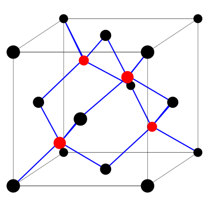
Si has the same crystal structure as Diamond:
a face-centered cubic lattice with two atoms in
the unit cell. In the figure, the black and red
dots identify the two sublattices. The side of
the cube is the lattice parameter a0. In the Di-
amond structure, the two sublattices have the
same composition; in the zincblende structure
(e.g. GaAs), they have different composition.
1http://www.fisica.uniud.it/%7Egiannozz/Corsi/MQ/Software/F90/cohenbergstresser.f90
2http://www.fisica.uniud.it/%7Egiannozz/Corsi/MQ/Software/C/cohenbergstresser.c
76
The origin of the coordinate system is arbitrary; typical choices are one of
the atoms, or the middle point between two neighboring atoms. We use the
latter choice because it yields inversion symmetry. The two atoms in the unit
cell are thus at positions d1 = −d, d2 = +d, where
1 1 1
d = a0
, ,
.
(10.10)
8 8 8
The lattice parameter for Si is a0 = 10.26 a.u.. 3
Let us re-examine the matrix elements between plane waves of a potential
V , given by a sum of spherical symmetric potentials Vµ centered around atomic
positions:
V (r) =
Vµ(|r − dµ − Rn|)
(10.13)
n
µ
With some algebra, one finds:
1
bi,k|V |bj,k =
V (r)e−iG·rdr = VSi(G) cos(G · d),
(10.14)
Ω Ω
where G = Gi − Gj. The cosine term is a special case of a geometrical factor
known as structure factor, while VSi(G) is known as the atomic form factor:
1
VSi(G) =
VSi(r)e−iG·rdr.
(10.15)
Ω Ω
Cohen-Bergstresser pseudopotentials are given as atomic form factors for a few
values of |G|, corresponding to the smallest allowed modules: G2 = 0, 3, 4, 8, 11, ...,
in units of (2π/a0)2.
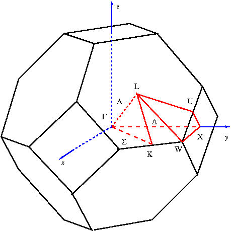
The code requires on input the cutoff (in Ry) for the kinetic energy of plane
waves, and a list of vectors k in the Brillouin Zone. Traditionally these points
are chosen along high-symmetry lines, joining high-symmetry points shown in
figure and listed below:
Γ
=
(0, 0, 0),
2π
X
=
(1, 0, 0),
a0
2π
1
W
=
(1, , 0),
a0
2
2π 3 3
K
=
( , , 0),
a0 4 4
2π 1 1 1
L
=
( , , ),
a0 2 2 2
3 We remark that the face-centered cubic lattice can also be described as a simple-cubic
lattice:
a1 = a0 (1, 0, 0) ,
a2 = a0 (0, 1, 0) ,
a3 = a0 (0, 0, 1)
(10.11)
with four atoms in the unit cell, at positions:
1 1
1
1
1 1
d1 = a0 0,
,
,
d2 = a0
, 0,
,
d3 = a0
,
, 0 ,
d4 = (0, 0, 0) .
(10.12)
2 2
2
2
2 2
77
10.3.1
Laboratory
• Verify which cutoff is needed to achieve converged results for E(k)
• Reproduce the results in the original paper for Si, Ge, Sn.
• Try to figure out what the charge density would be by plotting the sum
of the four lowest wavefunctions squared at the Γ point. It is convenient
to plot along the (110) plane (that is: one axis along (1,1,0), the other
along (0,0,1) ).
• In the zincblende lattice, the two atoms are not identical. Cohen and
Bergstresser introduce a “symmetric” and an “antisymmetric” contribu-
tion, corresponding respectively to a cosine and a sine times the imaginary
unit in the structure factor:
bi,k|V |bj,k = Vs(G) cos(G · d) + iVa(G) sin(G · d).
(10.16)
What do you think is needed in order to extend the code to cover the case
of Zincblende lattices?
78
Chapter 11
Exact diagonalization of
quantum spin models
Systems of interacting spins are used since many years to model magnetic phe-
nomena. Their usefulness extends well beyond the field of magnetism, since
many different physical phenomena can be mapped, exactly or approximately,
onto spin systems. Many models exists and many techniques can be used to
determine their properties under various conditions. In this chapter we will deal
with the exact solution (i.e. finding the ground state) for the Heisenberg model,
i.e. a quantum spin model in which spin centered at lattice sites interact via
the exchange interaction. The hyper-simplified model we are going to study is
sufficient to give an idea of the kind of problems one encounters when trying to
solve many-body systems without resorting to mean-field approximations (i.e.
reducing th