Using the circular convolution algorithms described above, we can easily design algorithms for prime length FFTs. The only modifications that needs to be made involve the permutation of Rader 5 and the correct calculation of the DC term (y(0)). These modifications are easily made to the above described approach. It simply requires a few extra commands in the programs. Note that the multiplicative constants are computed directly, since we have programs for all the relevant operations.

In the version we have currently implemented and verified for correctness, we precompute the multiplicative constants, the input permutation and the output permutation. From Equation 8 from A Bilinear Form for the DFT, the multiplicative constants are given by , the input permutation is given by 1⊕PQ_r, and the output permutation is given by 1⊕Q_s^tJP^t. The multiplicative constants, the input and output permutation are each stored as vectors. These vectors are then passed to the prime length FFT program, which consists of the appropriate function calls, see the appendix. In previous prime length FFT modules, the input and output permutations can be completely absorbed in to the computational instructions. This is possible because they are written as straight line code. It is simple to modify the code generating program we have implemented so that it produces straight line code and absorbs the permutations in to the computational program instructions.

In an in-place in-order prime factor algorithm for the DFT 1, 6, the necessary permuted forms of the DFT can be obtained by modifying the multiplicative constants. This can be easily done by permuting the roots of unity, w, in the expression for the multiplicative constants 1, 3, nothing else in the structure of the algorithm needs to be changed. By changing the multiplicative constants, it is not possible, however, to omit the permutation required for Rader's conversion of the prime length DFT in to circular convolution.

Operation Counts

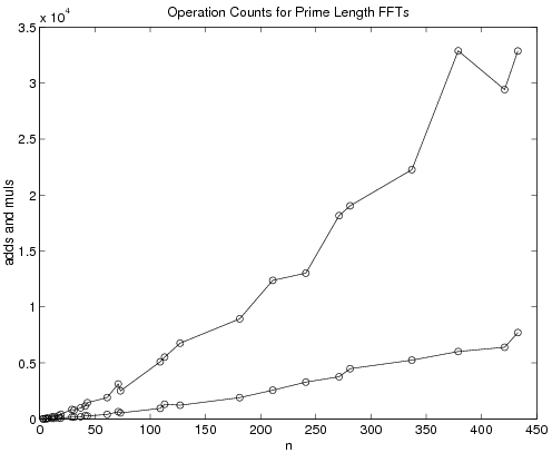
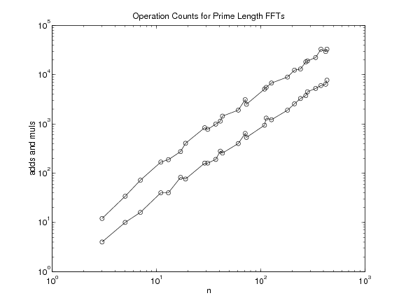
Table 7.1 lists the arithmetic operations incurred by the FFT programs we have generated and verified for correctness. Note that the number of additions and multiplications incurred by the programs we have generated are the same as previously existing programs for prime lengths up to and including 13. For p=17 a program with 70 multiplications and 314 additions has been written, and for p=19 a program with 76 multiplications and 372 additions has been written 2. Thus for the length p=17, the program we have generated requires fewer total arithmetic operations, while for p=19, ours uses more.

There are several table of operation counts in 4, each table corresponding to a different variation of the algorithms used in that paper. For each variation, the algorithms we have described use fewer additions and fewer multiplications. The focus of 4, however, is the implementation of prime point FFT on various computer architectures and the advantage that can be gained from matching algorithms with architectures. It should be noted that the highest prime in 4 for which an FFT was designed is 29. Although we have not executed the programs described in this paper on these computers, they are, as mentioned above, written to be easily adapted to parallel/vector computers.

Table 7.1. Operation counts for prime length FFTs

P	muls	adds		P	muls	adds		P	muls	adds
3	4	12		41	280	1140		241	3280	13020
5	10	34		43	256	1440		271	3760	18152
7	16	72		61	400	1908		281	4480	19036
11	40	168		71	640	3112		337	5248	22268
13	40	188		73	532	2504		379	6016	32880
17	82	274		109	940	5096		421	6400	29412
19	76	404		113	1312	5516		433	7708	32864
29	160	836		127	1216	6760		541	9400	43020
31	160	776		181	1900	8936		631	12160	56056
37	190	990		211	2560	12368		757	15040	76292

Figure 7.1. 

Plot of additions and multiplications incurred by prime length FFTs.

Figure 7.2. 

Plot of additions and multiplications incurred by prime length FFTs.