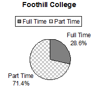
71.4%
Total
14,183
100%
Table 1.2
Tables are a good way of organizing and displaying data. But graphs can be even more helpful in
understanding the data. There are no strict rules concerning what graphs to use. Below are pie charts and
bar graphs, two graphs that are used to display qualitative data.
In a pie chart, categories of data are represented by wedges in the circle and are proportional in size
to the percent of individuals in each category.
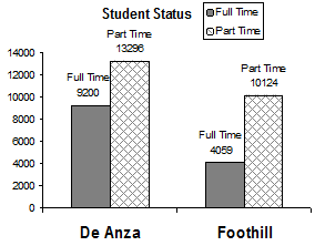
In a bar graph, the length of the bar for each category is proportional to the number or percent of
individuals in each category. Bars may be vertical or horizontal.
A Pareto chart consists of bars that are sorted into order by category size (largest to smallest).
Look at the graphs and determine which graph (pie or bar) you think displays the comparisons bet-
ter. This is a matter of preference.
It is a good idea to look at a variety of graphs to see which is the most helpful in displaying the
data. We might make different choices of what we think is the "best" graph depending on the data and the
context. Our choice also depends on what we are using the data for.
Available for free at Connexions <http://cnx.org/content/col10522/1.40>
21
Table 1.3
Table 1.4
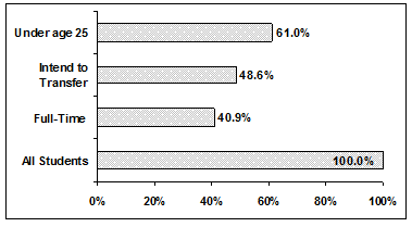
Percentages That Add to More (or Less) Than 100%
Sometimes percentages add up to be more than 100% (or less than 100%). In the graph, the percentages
add to more than 100% because students can be in more than one category. A bar graph is appropriate
to compare the relative size of the categories. A pie chart cannot be used. It also could not be used if the
percentages added to less than 100%.
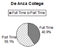
De Anza College Spring 2010
Characteristic/Category
Percent
Full-time Students
40.9%
Students who intend to transfer to a 4-year educational institution
48.6%
Students under age 25
61.0%
TOTAL
150.5%
Table 1.5
Available for free at Connexions <http://cnx.org/content/col10522/1.40>
22
CHAPTER 1. SAMPLING AND DATA
Table 1.6
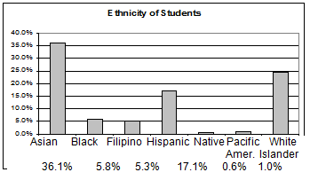
Omitting Categories/Missing Data
The table displays Ethnicity of Students but is missing the "Other/Unknown" category. This category con-
tains people who did not feel they fit into any of the ethnicity categories or declined to respond. Notice that
the frequencies do not add up to the total number of students. Create a bar graph and not a pie chart.
Missing Data: Ethnicity of Students De Anza College Fall Term 2007 (Census Day)
Frequency
Percent
Asian
8,794
36.1%
Black
1,412
5.8%
Filipino
1,298
5.3%
Hispanic
4,180
17.1%
Native American
146
0.6%
Pacific Islander
236
1.0%
White
5,978
24.5%
TOTAL
22,044 out of 24,382
90.4% out of 100%
Table 1.7
Available for free at Connexions <http://cnx.org/content/col10522/1.40>
23
Bar graph Without Other/Unknown Category
Table 1.8
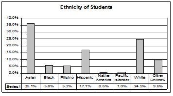
The following graph is the same as the previous graph but the "Other/Unknown" percent (9.6%) has been
added back in. The "Other/Unknown" category is large compared to some of the other categories (Native
American, 0.6%, Pacific Islander 1.0% particularly). This is important to know when we think about what
the data are telling us.
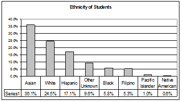
This particular bar graph can be hard to understand visually. The graph below it is a Pareto chart.
The Pareto chart has the bars sorted from largest to smallest and is easier to read and interpret.
Bar Graph With Other/Unknown Category
Table 1.9
Available for free at Connexions <http://cnx.org/content/col10522/1.40>
24
CHAPTER 1. SAMPLING AND DATA
Pareto Chart With Bars Sorted By Size
Table 1.10
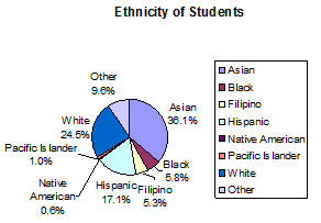
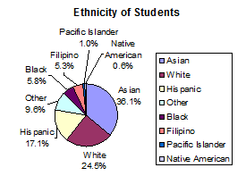
Pie Charts: No Missing Data
The following pie charts have the "Other/Unknown" category added back in (since the percentages must
add to 100%). The chart on the right is organized having the wedges by size and makes for a more visually
informative graph than the unsorted, alphabetical graph on the left.
Table 1.11
1.6 Sampling6
Gathering information about an entire population often costs too much or is virtually impossible. Instead,
we use a sample of the population. A sample should have the same characteristics as the population it
is representing. Most statisticians use various methods of random sampling in an attempt to achieve this
goal. This section will describe a few of the most common methods.
There are several different methods of random sampling. In each form of random sampling, each member
of a population initially has an equal chance of being selected for the sample. Each method has pros and
cons. The easiest method to describe is called a simple random sample. Any group of n individuals is
6This content is available online at <http://cnx.org/content/m16014/1.17/>.
Available for free at Connexions <http://cnx.org/content/col10522/1.40>
25
equally likely to be chosen by any other group of n individuals if the simple random sampling technique is
used. In other words, each sample of the same size has an equal chance of being selected. For example, sup-
pose Lisa wants to form a four-person study group (herself and three other people) from her pre-calculus
class, which has 31 members not including Lisa. To choose a simple random sample of size 3 from the other
members of her class, Lisa could put all 31 names in a hat, shake the hat, close her eyes, and pick out 3
names. A more technological way is for Lisa to first list the last names of the members of her class together
with a two-digit number as shown below.
Available for free at Connexions <http://cnx.org/content/col10522/1.40>
26
CHAPTER 1. SAMPLING AND DATA
Class Roster
ID
Name
00
Anselmo
01
Bautista
02
Bayani
03
Cheng
04
Cuarismo
05
Cuningham
06
Fontecha
07
Hong
08
Hoobler
09
Jiao
10
Khan
11
King
12
Legeny
13
Lundquist
14
Macierz
15
Motogawa
16
Okimoto
17
Patel
18
Price
19
Quizon
20
Reyes
21
Roquero
22
Roth
23
Rowell
24
Salangsang
25
Slade
26
Stracher
27
Tallai
28
Tran
29
Wai
30
Wood
Table 1.12
Lisa can either use a table of random numbers (found in many statistics books as well as mathematical
handbooks) or a calculator or computer to generate random numbers. For this example, suppose Lisa
chooses to generate random numbers from a calculator. The numbers generated are:
Available for free at Connexions <http://cnx.org/content/col10522/1.40>
27
.94360; .99832; .14669; .51470; .40581; .73381; .04399
Lisa reads two-digit groups until she has chosen three class members (that is, she reads .94360 as the groups
94, 43, 36, 60). Each random number may only contribute one class member. If she needed to, Lisa could
have generated more random numbers.
The random numbers .94360 and .99832 do not contain appropriate two digit numbers. However the third
random number, .14669, contains 14 (the fourth random number also contains 14), the fifth random number
contains 05, and the seventh random number contains 04. The two-digit number 14 corresponds to Macierz,
05 corresponds to Cunningham, and 04 corresponds to Cuarismo. Besides herself, Lisa’s group will consist
of Marcierz, and Cunningham, and Cuarismo.
Besides simple random sampling, there are other forms of sampling that involve a chance process for get-
ting the sample. Other well-known random sampling methods are the stratified sample, the cluster
sample, and the systematic sample.
To choose a stratified sample, divide the population into groups called strata and then take a proportionate
number from each stratum. For example, you could stratify (group) your college population by department
and then choose a proportionate simple random sample from each stratum (each department) to get a strat-
ified random sample. To choose a simple random sample from each department, number each member of
the first department, number each member of the second department and do the same for the remaining de-
partments. Then use simple random sampling to choose proportionate numbers from the first department
and do the same for each of the remaining departments. Those numbers picked from the first department,
picked from the second department and so on represent the members who make up the stratified sample.
To choose a cluster sample, divide the population into clusters (groups) and then randomly select some of
the clusters. All the members from these clusters are in the cluster sample. For example, if you randomly
sample four departments from your college population, the four departments make up the cluster sample.
For example, divide your college faculty by department. The departments are the clusters. Number each
department and then choose four different numbers using simple random sampling. All members of the
four departments with those numbers are the cluster sample.
To choose a systematic sample, randomly select a starting point and take every nth piece of data from a
listing of the population. For example, suppose you have to do a phone survey. Your phone book contains
20,000 residence listings. You must choose 400 names for the sample. Number the population 1 - 20,000
and then use a simple random sample to pick a number that represents the first name of the sample. Then
choose every 50th name thereafter until you have a total of 400 names (you might have to go back to the of
your phone list). Systematic sampling is frequently chosen because it is a simple method.
A type of sampling that is nonrandom is convenience sampling. Convenience sampling involves using
results that are readily available. For example, a computer software store conducts a marketing study by
interviewing potential customers who happen to be in the store browsing through the available software.
The results of convenience sampling may be very good in some cases and highly biased (favors certain
outcomes) in others.
Sampling data should be done very carefully. Collecting data carelessly can have devastating results. Sur-
veys mailed to households and then returned may be very biased (for example, they may favor a certain
group). It is better for the person conducting the survey to select the sample respondents.
True random sampling is done with replacement. That is, once a member is picked that member goes
back into the population and thus may be chosen more than once. However for practical reasons, in most
populations, simple random sampling is done without replacement. Surveys are typically done without
replacement. That is, a member of the population may be chosen only once. Most samples are taken from
large populations and the sample tends to be small in comparison to the population. Since this is the case,
Available for free at Connexions <http://cnx.org/content/col10522/1.40>
28
CHAPTER 1. SAMPLING AND DATA
sampling without replacement is approximately the same as sampling with replacement because the chance
of picking the same individual more than once using with replacement is very low.
For example, in a college population of 10,000 people, suppose you want to randomly pick a sample of 1000
for a survey. For any particular sample of 1000, if you are sampling with replacement,
• the chance of picking the first person is 1000 out of 10,000 (0.1000);
• the chance of picking a different second person for this sample is 999 out of 10,000 (0.0999);
• the chance of picking the same person again is 1 out of 10,000 (very low).
If you are sampling without replacement,
• the chance of picking the first person for any particular sample is 1000 out of 10,000 (0.1000);
• the chance of picking a different second person is 999 out of 9,999 (0.0999);
• you do not replace the first person before picking the next person.
Compare the fractions 999/10,000 and 999/9,999. For accuracy, carry the decimal answers to 4 place deci-
mals. To 4 decimal places, these numbers are equivalent (0.0999).
Sampling without replacement instead of sampling with replacement only becomes a mathematics issue
when the population is small which is not that common. For example, if the population is 25 people, the
sample is 10 and you are sampling with replacement for any particular sample,
• the chance of picking the first person is 10 out of 25 and a different second person is 9 out of 25 (you
replace the first person).
If you sample without replacement,
• the chance of picking the first person is 10 out of 25 and then the second person (which is different) is
9 out of 24 (you do not replace the first person).
Compare the fractions 9/25 and 9/24. To 4 decimal places, 9/25 = 0.3600 and 9/24 = 0.3750. To 4 decimal
places, these numbers are not equivalent.
When you analyze data, it is important to be aware of sampling errors and nonsampling errors. The actual
process of sampling causes sampling errors. For example, the sample may not be large enough. Factors
not related to the sampling process cause nonsampling errors. A defective counting device can cause a
nonsampling error.
In reality, a sample will never be exactly representative of the population so there will always be
some sampling error. As a rule, the larger the sample, the smaller the sampling error.
In statistics, a sampling bias is created when a sample is collected from a population and some
members of the population are not as likely to be chosen as others (remember, each member of the
population should have an equally likely chance of being chosen). When a sampling bias happens, there
can be incorrect conclusions drawn about the population that is being studied.
Example 1.6
Determine the type of sampling used (simple random, stratified, systematic, cluster, or conve-
nience).
1. A soccer coach selects 6 players from a group of boys aged 8 to 10, 7 players from a group of
boys aged 11 to 12, and 3 players from a group of boys aged 13 to 14 to form a recreational
soccer team.
2. A pollster interviews all human resource personnel in five different high tech companies.
Available for free at Connexions <http://cnx.org/content/col10522/1.40>
29
3. A high school educational researcher interviews 50 high school female teachers and 50 high
school male teachers.
4. A medical researcher interviews every third cancer patient from a list of cancer patients at a
local hospital.
5. A high school counselor uses a computer to generate 50 random numbers and then picks
students whose names correspond to the numbers.
6. A student interviews classmates in his algebra class to determine how many pairs of jeans a
student owns, on the average.
Solution
1. stratified
2. cluster
3. stratified
4. systematic
5. simple random
6. convenience
If we were to examine two samples representing the same population, even if we used random sampling
methods for the samples, they would not be exactly the same. Just as there is variation in data, there is
variation in samples. As you become accustomed to sampling, the variability will seem natural.
Example 1.7
Suppose ABC College has 10,000 part-time students (the population). We are interested in the
average amount of money a part-time student spends on books in the fall term. Asking all 10,000
students is an almost impossible task.
Suppose we take two different samples.
First, we use convenience sampling and survey 10 students from a first term organic chemistry
class. Many of these students are taking first term calculus in addition to the organic chemistry
class . The amount of money they spend is as follows:
$128; $87; $173; $116; $130; $204; $147; $189; $93; $153
The second sample is taken by using a list from the P.E. department of senior citizens who take
P.E. classes and taking every 5th senior citizen on the list, for a total of 10 senior citizens. They
spend:
$50; $40; $36; $15; $50; $100; $40; $53; $22; $22
Problem 1
Do you think that either of these samples is representative of (or is characteristic of) the entire
10,000 part-time student population?
Solution
No. The first sample probably consists of science-oriented students. Besides the chemistry course,
some of them are taking first-term calculus. Books for these classes tend to be expensive. Most
of these students are, more than likely, paying more than the average part-time student for their
books. The second sample is a group of senior citizens who are, more than likely, taking courses
for health and interest. The amount of money they spend on books is probably much less than the
average part-time student. Both samples are biased. Also, in both cases, not all students have a
chance to be in either sample.
Available for free at Connexions <http://cnx.org/content/col10522/1.40>
30
CHAPTER 1. SAMPLING AND DATA
Problem 2
Since these samples are not representative of the entire population, is it wise to use the results to
describe the entire population?
Solution
No. For these samples, each member of the population did not have an equally likely chance of
being chosen.
Now, suppose we take a third sample. We choose ten different part-time students from the dis-
ciplines of chemistry, math, English, psychology, sociology, history, nursing, physical education,
art, and early childhood development. (We assume that these are the only disciplines in which
part-time students at ABC College are enrolled and that an equal number of part-time students
are enrolled in each of the disciplines.) Each student is chosen using simple random sampling.
Using a calculator, random numbers are generated and a student from a particular discipline is
selected if he/she has a corresponding number. The students spend:
$180; $50; $150; $85; $260; $75; $180; $200; $200; $150
Problem 3
Is the sample biased?
Solution
The sample is unbiased, but a larger sample would be recommended to increase the likelihood
that the sample will be close to representative of the population. However, for a biased sampling
technique, even a large sample runs the risk of not being representative of the population.
Students often ask if it is "good enough" to take a sample, instead of surveying the entire popula-
tion. If the survey is done well, the answer is yes.
1.6.1 Optional Collaborative Classroom Exercise
Exercise 1.6.1
As a class, determine whether or not the following samples are representative. If they are not,
discuss the reasons.
1. To find the average GPA of all students in a university, use all honor students at the univer-
sity as the sample.
2. To find out the most popular cereal among young people under the age of 10, stand outside
a large supermarket for three hours and speak to every 20th child under age 10 who enters
the supermarket.
3. To find the average annual income of all adults in the United States, sample U.S. congress-
men. Create a cluster sample by considering each state as a stratum (group). By using simple
random sampling, select states to be part of the cluster. Then survey every U.S. congressman
in the cluster.
4. To determine the proportion of people taking public transportation to work, survey 20 peo-
ple in New York City. Conduct the survey by sitting in Central Park on a bench and inter-
viewing every person who sits next to you.
5. To determine the average cost of a two day stay in a hospital in Massachusetts, survey 100
hospitals across the state using simple random sampling.
Available for free at Connexions <http://cnx.org/content/col10522/1.40>
31
1.7 Variation7
1.7.1 Variation in Data
Variation is present in any set of data. For example, 16-ounce cans of beverage may contain more or less
than 16 ounces of liquid. In one study, eight 16 ounce cans were measured and produced the following
amount (in ounces) of beverage:
15.8; 16.1; 15.2; 14.8; 15.8; 15.9; 16.0; 15.5
Measurements of the amount of beverage in a 16-ounce can may vary because different people make the
measurements or because the exact amount, 16 ounces of liquid, was not put into the cans. Manufacturers
regularly run tests to determine if the amount of beverage in a 16-ounce can falls within the desired range.
Be aware that as you take data, your data may vary somewhat from the data someone else is taking for the
same purpose. This is completely natural. However, if two or more of you are taking the same data and
get very different results, it is time for you and the others to reevaluate your data-taking methods and your
accuracy.
1.7.2 Variation in Samples
It was mentioned previously that two or more samples from the same population, taken randomly, and
having close to the same characteristics of the population are different from each other. Suppose Doreen and
Jung both decide to study the average amount of time students at their college sleep each night. Doreen and
Jung each take samples of 500 students. Doreen uses systematic sampling and Jung uses cluster sampling.
Doreen’s sample will be different from Jung’s sample. Even if Doreen and Jung used the same sampling
method, in all likelihood their samples would be different. Neither would be wrong, however.
Think about what contributes to making Doreen?