The first issue is to decide which of the four Fourier transforms to apply. This is easy,
since there is only one of the four that is computable, the DFT. Since we do not have an
analytic expression for the speech signal, we cannot algebraically determine the DTFT.
However, we know from the previous section that the DFT yields samples of the DTFT
of a finite signal, so calculating the DFT reveals the structure of the DTFT.
The DFT of these 512 samples is shown at the bottom in Figure 10.11, which shows
one cycle of the periodic DFT. The horizontal axis is labeled with the frequecies in Hz
rather than the index k of the DFT coefficient. Recall that the k-th coefficient of the
DFT represents a complex exponential with frequency kω0 = k2π/p radians/sample. To
convert this to Hertz, we watch the units,
(k2π/p)[radians/sample] × (1/T )[samples/second] × (1/2π)[cycles/radian]
= k/(pT )[cycles/second],
where T = 1/8000 is the sampling interval.
Although this plot shows the DFT, the plot can equally well be interpreted as a plot of
the DTFT. It shows 512 values of the DFT (one cycle of the periodic signal), and instead
of showing each individual value, it runs them together as a continuous curve. In fact,
since the DFT is samples of the DTFT, that continuous curve is a pretty good estimate
of the shape of the DTFT. Of course, the samples might not be close together enough to
accurately represent the DTFT, but probably they are. The next chapter will examine this
issue in considerable detail.
Notice that most of the signal is concentrated below 1 kHz. In Figure 10.12, we have
zoomed in to this region of the spectrum. Notice that the DFT is strongly peaked, with
the lowest frequency peak occurring at about 120 Hz. Indeed, this is not surprising,
because the time-domain signal at the top of Figure 10.11 looks somewhat periodic, with
a period of about 80 msec, roughly the inverse of 120 Hz. That is, it looks like a periodic
signal with fundamental frequency 120 Hz, and various harmonics. The weights of the
harmonics are proportional to the heights of the peaks in Figure 10.12.
The vowel in the word “sound” is created by vibrating the human vocal chords, and then
shaping the mouth into an acoustic cavity that alters the sound produced by the vocal
chords. A sound that uses the vocal chords is called by linguists a voiced sound. By
contrast, the “s” in “this” is an unvoiced sound. It is created without the help of the vocal
chords by forcing air through a narrow passage in the mouth to create turbulence.
The “s” in “this” is shown in Figure 10.13. It is very different from the vowel sound in
10.11. In particular, it looks much less regular. There is no evident periodicity in the
436
Lee & Varaiya, Signals and Systems
10. THE FOUR FOURIER TRANSFORMS
30
20
10
magnitude DFT
0
-1000 -800 -600 -400 -200
0
200
400
600
800
1000
frequency (in Hz)
Figure 10.12: DFT of the voiced segment of speech, shown over a narrower
frequency range.
signal, so the DFT does not reveal a fundamental frequency and harmonics. It is a noise-
like signal, where the DFT reveals that much of the noise is at low frequencies, below 500
Hz, but there are also significant components all the way out to 4 kHz.
The analysis we have done on the segments of speech is a typical use of Fourier analysis.
A long (even infinite) signal is divided into short segments, such as the two 512-sample
segments that we examined above. These segments are studied by calculating their DFT.
Since the DFT is a finite summation, it is easy to realize on a computer. Also, as men-
tioned before, there is a highly efficient algorithm called the fast Fourier transform or
FFT to calculate the DFT. The fft function in Matlab was used to calculate the DFTs
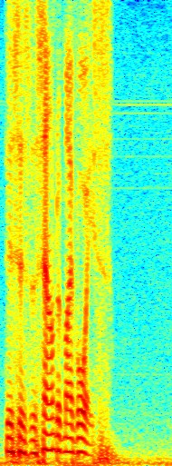
in figures 10.11 and 10.13. The DFT yields samples of the DTFT of the finite segment of signal. The spectrogram for the signal in Figure 10.10 is shown in Figure 10.14.
10.6.3
Fourier transforms of periodic signals
In the previous two sections, we have seen the relationship between the DTFT of a finite
signal and the DFT of the periodic signal that is constructed by repeating the finite signal.
The periodic signal, however, also has a DTFT itself. In the interest of variety, we will
explore this concept in continuous time.
Lee & Varaiya, Signals and Systems
437
10.6. FOURIER TRANSFORMS VS. FOURIER SERIES
0.1
0
amplitude -0.1
-0.2
0.01
0.02
0.03
0.04
0.05
0.06
time (in seconds)
10
8
6
4
magnitude DFT
2
0
-4000
-3000
-2000
-1000
0
1000
2000
3000
4000
frequency (in Hz)
Figure 10.13: An unvoiced segment of speech (top) and one cycle of the magni-
tude of its DFT (bottom).
438
Lee & Varaiya, Signals and Systems
10. THE FOUR FOURIER TRANSFORMS
4000
3000
2000
Frequency
1000
0 0
0.5
1
1.5
2
2.5
Time
1
0.5
0
−0.5
−10
0.5
1
1.5
2
2.5
4
x 10
Figure 10.14: Spectrogram of the voice segment in Figure 10.10.
Lee & Varaiya, Signals and Systems
439
10.6. FOURIER TRANSFORMS VS. FOURIER SERIES
A periodic continuous-time signal has a Fourier transform. But, as we will see, that
Fourier transform has Dirac delta functions in it, which are mathematically tricky. Recall
that a Dirac delta function is an infinitely narrow and infinitely high pulse. The Fourier
series permits us to talk about the frequency domain representation of a periodic signal
without dealing with Dirac delta functions.
It is useful, certainly, to simplify the mathematics. Using a Fourier series whenever pos-
sible allows us to do that. Moreover, when working with signals computationally, ev-
erything must be discrete and finite. Computers cannot deal with infinitely narrow and
infinitely high pulses numerically. Computation, therefore, must be done with the only
transform that is completely discrete and finite, the DFS, or its scaled cousin, the DFT.
To be concrete, suppose a continuous-time signal x has Fourier transform
∀ ω ∈ R, X(ω) = 2πδ(ω − ω0)
(10.15)
for some real value ω0. We can find x using the inverse CTFT (10.14),
∞
Z
∀
1
t ∈ R,
x(t) =
2πδ(ω − ω0)eiωtdω.
2π−∞
Using the sifting rule, this evaluates to
x(t) = eiω0t .
This is a periodic function with period p = 2π/ω0. From table 10.1, we see that the
Fourier series for x is
∀
1
if m = 1
m ∈ Z,
Xm =
0
otherwise
There is exactly one non-zero Fourier series coefficient, which corresponds to the exactly
one Dirac delta pulse in the Fourier transform (10.15).
More generally, suppose x has multiple Dirac delta pulses in its Fourier transform, each
with different weights,
∞
∀ ω ∈ R, X(ω) = 2π ∑ Xmδ(ω − mω0).
(10.16)
m=−∞
The inverse CTFT (10.14) tells us that
∞
∀ t ∈ R, x(t) = ∑ Xmeimω0t.
m=−∞
440
Lee & Varaiya, Signals and Systems
10. THE FOUR FOURIER TRANSFORMS
X(!)
"
"
!
#!
!
0
0
Figure 10.15: Fourier transform of a cosine.
This is a periodic function with fundamental frequency ω0, and harmonics in various
weights. Its Fourier series coefficients, by inspection, are just Xm. Thus, for a periodic
signal, (10.16) relates the CTFT and the Fourier series. The Fourier series gives the
weights of a set of Dirac delta pulses in the Fourier transform, within a scaling factor of
2π.
Example 10.5: Consider x given by
∀ t ∈ R, x(t) = cos(ω0t).
From table 10.1, we see that the Fourier series for x is
∀
1/2 if |m| = 1
m ∈ Z,
Xm =
0
otherwise
There are only two non-zero Fourier series coefficients. We can use (10.16) to write
down its Fourier transform,
∀ ω ∈ R, X(ω) = πδ(ω + ω0) + πδ(ω − ω0).
We sketch this as shown in Figure 10.15. See Exercise 9 at the end of the chapter for a similar result for a sin function.
Lee & Varaiya, Signals and Systems
441
10.7. PROPERTIES OF FOURIER TRANSFORMS
| X(!)|
"
2
2/3 2/5 2/7 !
!0 3!0
Figure 10.16: Fourier transform of a square wave.
Example 10.6:
Consider the square wave of example 10.1. The Fourier series
coefficients are
1/2
if m = 0
Xm =
0
if m is even and m = 0
−i/mπ if m is odd
The Fourier transform, therefore, has Dirac delta pulses with these weights at mul-
tiples of ω0, scaled by 2π, as shown in Figure 10.16.
The same concept applies in the discrete-time case, although some care is needed because
the DTFT and DFT are both periodic, and not every function of the form e jωn is periodic
(see Section 7.6.1). In fact, in Figure 10.11, the peaks in the spectrum hint at the Dirac delta functions in the DTFT. The signal appears to be roughly periodic with period 120
Hz, so the DFT shows strong peaks at multiples of 120 Hz. If the signal were perfectly
periodic, and if we were plotting the DTFT instead of the DFT, then these peaks would
become infinitely narrow and infinitely high.
10.7
Properties of Fourier transforms
In this section, we give a number of useful properties of the various Fourier transforms,
together with a number of illustrative examples. These properties are summarized in
tables 10.6 through 10.9. The properties and examples can often be used to avoid solving 442
Lee & Varaiya, Signals and Systems
10. THE FOUR FOURIER TRANSFORMS
Time domain
Frequency domain
Reference
∀ t ∈ R, x(t) is real
∀ m ∈ Z, Xm = X∗−m
Section
∀ t ∈ R, x(t) = x∗(−t)
∀ m ∈ Z, Xm is real
Section
∀ t ∈ R, y(t) = x(t − τ)
∀ m ∈ Z, Ym = e−imω0τXm
Section
∀ t ∈ R, y(t) = eiω1tx(t)
∀ m ∈ Z, Ym = Xm−M
Section
where ω1 = Mω0, for some M ∈ Z
∀ t ∈ R,
∀ m ∈ Z,
Example
y(t) = cos(ω1t)x(t)
Ym = (Xm−M + Xm+M)/2
where ω1 = Mω0, for some M ∈ Z
∀ t ∈ R,
∀ m ∈ Z,
Exercise
y(t) = sin(ω1t)x(t)
Ym = (Xm−M − Xm+M)/2i
where ω1 = Mω0, for some M ∈ Z
∀ t ∈ R,
∀ m ∈ Z,
Section
y(t) = ax(t) + bw(t)
Ym = aXm + bWm
∀ t ∈ R, y(t) = x∗(t)
∀ m ∈ Z, Ym = X∗−m
–
Table 10.6: Properties of the Fourier series. All time-domain signals are assumed
to be periodic with period p, and fundamental frequency ω0 = 2π/p.
Lee & Varaiya, Signals and Systems
443
10.7. PROPERTIES OF FOURIER TRANSFORMS
Time domain
Frequency domain
Reference
∀ n ∈ Z, x(n) is real
∀ k ∈ Z, X = X ∗
Section
k
−k
∀ n ∈ Z, x(n) = x∗(−n)
∀ k ∈ Z, X is real
Section
k
∀ n ∈ Z, y(n) = x(n − N)
∀ k ∈ Z, Y = e−ikω0NX
–
k
k
∀ n ∈ Z, y(n) = eiω1nx(n)
∀ k ∈ Z, Y = X
–
k
k−M
where ω1 = Mω0, for some M ∈ Z
∀ n ∈ Z,
∀ k ∈ Z,
–
y(n) = cos(ω1n)x(n)
Y = (X
+ X
)/2
k
k−M
k+M
where ω1 = Mω0, for some M ∈ Z
∀ n ∈ Z,
∀ k ∈ Z,
–
y(n) = sin(ω1n)x(n)
Y = (X
− X
)/2i
k
k−M
k+M
where ω1 = Mω0, for some M ∈ Z
∀ n ∈ Z,
∀ k ∈ Z,
Section
y(n) = ax(n) + bw(n)
Y = aX + bW
k
k
k
∀ n ∈ Z, y(n) = x∗(n)
∀ k ∈ Z, Yk = X∗−
–
k
Table 10.7: Properties of the DFT. All time-domain signals are assumed to be
periodic with period p, and fundamental frequency ω0 = 2π/p.
444
Lee & Varaiya, Signals and Systems
10. THE FOUR FOURIER TRANSFORMS
Time domain
Frequency domain
Reference
∀ n ∈ Z, x(n) is real
∀ ω ∈ R, X(ω) = X∗(−ω)
Section
∀ n ∈ Z, x(n) = x∗(−n)
∀ ω ∈ R, X(ω) is real
Section
∀ n ∈ Z, y(n) = x(n − N)
∀ ω ∈ R, Y(ω) = e−iωNX(ω)
Section
∀ n ∈ Z, y(n) = eiω1nx(n)
∀ ω ∈ R, Y(ω) = X(ω − ω1)
Section
∀ n ∈ Z,
∀ ω ∈ R,
Example
y(n) = cos(ω1n)x(n)
Y (ω) = (X (ω − ω1) + X(ω + ω1))/2
∀ n ∈ Z,
∀ ω ∈ R,
Exercise
y(n) = sin(ω1n)x(n)
Y (ω) = (X (ω − ω1) − X(ω + ω1))/2i
∀ n ∈ Z,
∀ ω ∈ R,
Section
x(n) = ax1(n) + bx2(n)
X (ω) = aX1(ω) + bX2(ω)
∀ n ∈ Z, y(n) = (h ∗ x)(n)
∀ ω ∈ R, Y(ω) = H(ω)X(ω)
Section
∀ n ∈ Z, y(n) = x(n)p(n)
∀ ω ∈ R,
Box on
2π
page 457
Y (
R
ω) = 1
X (
2
Ω)P(ω − Ω)dΩ
π 0
∀ n ∈ Z,
∀ ω ∈ R,
Exercise
x(n/N) n multiple of N
Y (ω) = X (NΩ)
y(n) =
0
otherwise
Table 10.8: Properties of the DTFT.
Lee & Varaiya, Signals and Systems
445
10.7. PROPERTIES OF FOURIER TRANSFORMS
Time domain
Frequency domain
Reference
∀ t ∈ R, x(t) is real
∀ ω ∈ R, X(ω) = X∗(−ω)
Section
∀ t ∈ R, x(t) = x∗(−t)
∀ ω ∈ R, X(ω) is real
Section
∀ t ∈ R, y(t) = x(t − τ)
∀ ω ∈ R, Y(ω) = e−iωτX(ω)
Section
∀ t ∈ R, y(t) = eiω1tx(t)
∀ ω ∈ R, Y(ω) = X(ω − ω1)
Section
∀ t ∈ R,
∀ ω ∈ R,
Example
y(t) = cos(ω1t)x(t)
Y (ω) = (X (ω − ω1) + X(ω + ω1))/2
∀ t ∈ Z,
∀ ω ∈ R,
Exercise
y(t) = sin(ω1t)x(t)
Y (ω) = (X (ω − ω1) − X(ω + ω1))/2i
∀ t ∈ R,
∀ ω ∈ R,
Section
x(t) = ax1(t) + bx2(t)
X (ω) = aX1(ω) + bX2(ω)
∀ t ∈ R, y(t) = (h ∗ x)(t)
∀ ω ∈ R, Y(ω) = H(ω)X(ω)
Section
∀ t ∈ R, y(t) = x(t)p(t)
∀ ω ∈ R,
–
∞
Y (
R
ω) = 1
X (
2
Ω)P(ω − Ω)dΩ
π −∞
∀ t ∈ R,
∀ ω ∈ R,
Exercise
y(t) = x(at)
Y (ω) = 1
|
a| X (Ω/a)
Table 10.9: Properties of the CTFT.
446
Lee & Varaiya, Signals and Systems
10. THE FOUR FOURIER TRANSFORMS
integrals or summations to find the Fourier transform of some signal, or to find an inverse
Fourier transform.
10.7.1
Convolution
Suppose a discrete-time LTI system has impulse response h and frequency response H.
We have seen that if the input to this system is a complex exponential, eiωn, then the output
is H(ω)eiωn. Suppose the input is instead an arbitrary signal x with DTFT X . Using the
inverse DTFT relation, we know that
2π
Z
∀
1
n ∈ Z,
x(n) =
X (ω)eiωndω.
2π 0
View this as a summation of exponentials, each with weight X (ω). An integral, after all,
is summation over a continuum. Each term in the summation is X (ω)eiωn. If this term
were an input by itself, then the output would be H(ω)X (ω)eiωn. Thus, by linearity, if the
input is x, the output should be
2π
Z
∀
1
n ∈ Z,
y(n) =
H(ω)X (ω)eiωndω
2π 0
Comparing to the inverse DTFT relation for y(n), we see that
∀ ω ∈ R, Y(ω) = H(ω)X(ω).
(10.17)
This is the frequency-domain version of convolution
∀ n ∈ Z, y(n) = (h ∗ x)(n).
Thus, the frequency response of an LTI system multiplies the DTFT of the input. This is
intuitive, since the frequency response gives the weight imposed by the system on each
frequency component of the input.
Equation (10.17) applies equally well to continuous-time systems, but in that case, H is
the CTFT of the impulse response, and X is the CTFT of the input.
Lee & Varaiya, Signals and Systems
447
10.7. PROPERTIES OF FOURIER TRANSFORMS
10.7.2
Conjugate symmetry
We have already shown (see (8.29)) that for real-valued signals, the Fourier series coeffi-
cients are conjugate symmetric,
Xk = X∗
− .
k
In fact, all the Fourier transforms are conjugate symmetric if the time-domain function is
real.
We illustrate this with the CTFT. Suppose x : R → R is a real-valued signal, and
let X = CTFT(x). In general, X (ω) will be complex-valued. However, from (10.13), we
have
Z
∞
[X (−ω)]∗ =
[x(t)eiωt ]∗dt
−∞
Z
∞
=
x(t)e−iωt dt
−∞
=
X (ω),
Thus,
X (ω) = X ∗(−ω),
i.e. for real-valued signals, X (ω) and X (−ω) are complex conjugates of one another.
We can show that, conversely, if the Fourier transform is conjugate symmetric, then the
time-domain function is real. To do this, write the inverse CTFT
∞
1 Z
x(t) =
X (ω)eiωt dω
2π−∞
and then conjugate both sides,
∞
1 Z
x∗(t) =
X ∗(ω)e−iωt dω.
2π−∞
By changing variables (replacing ω with −ω) and using the conjugate symmetry of X, we
can show that
x∗(t) = x(t),
which implies that x(t) is real for all t.
The inverse Fourier transforms can be used to show that if a time-domain function is
conjugate symmetric,
x(t) = x∗(−t),
448