


From Dynamic Modeling to Experimentation of
Induction Motor Powered by Doubly-Fed Induction Generator by Passivity-Based Control
125
5.3 PBC + PI
The PBC + PI controller is given by the equation below:
BvrG = ˙ λd + RL− 1( θ) λd + B Kp( isG − id ) +
)
sG
Ki
( isG − idsG
(46)
where Kp and Ki are the proportional and integral positive gains. We have:
( isG − id ) = − 1( λ
)
sG
(47)
R
sG M − λdsGM
2
−
=
1
0
I
( λ − λd)
(48)
R
2
0
2
P
˜ λ
Then,
BvrG = ˙ λd + RL− 1( θ) λd + KpBPL− 1( θ) ˜ λ − Ki BP ˜ λ
(49)
R 2
The closed loop error dynamic is:
˙˜ λ = −RL− 1( θ)˜ λ − KpBPL− 1( θ)˜ λ + Ki BP˜ λ
(50)
R 2
Consider the desired energy function given by (33), it’s derivative along the trajectories of (50)
is:
˙
V
= ˜ λTR− 1 ˙˜ λ
= − ˜ λTL− 1( θ)˜ λ − K ˜
˜
p λT R− 1 BPL− 1( θ) ˜
λ + Ki λTR− 1 BP ˜ λ
R 2
= − ˜ λT L− 1( θ) ˜ λ + ˜ λT −K
˜
p R− 1 BPL− 1( θ) + Ki R− 1 BP λ
R 2
> 0
M
To show that the error dynamic (50) is stable, it’s enough to prove that M is a negative
semi-definite matrix:
⎡
⎤
Kp
Kp
⎢ − Kp
|Δ | LmG LrMeJnGθG
|Δ | LrG LrM + Ki I
R
2
2
|Δ | LrG LmMeJnMθM ⎥
M = 1 ⎣
⎦
(51)
R
0
0
0
1
0
0
0
M is a negative semi-definite matrix if: XT MX ≤ 0
X ∈ 6 × 1
⎡
⎤
− Kp
Kp
K
I
p
⎢
|Δ | LmG LrMeJnGθG
2 |Δ | LrG LrM + Ki
2 R
2
2
2 |Δ | LrG LmMeJnMθM ⎥
XT MX= 1 XT⎢
Kp
I
⎥ X
(52)
R
⎣ 2 |Δ | LrGLrM + Ki
2 R
2
0
0
⎦
1
2
Kp
2 |Δ | LrG LmMe−JnMθM
0
0
M
To prove that M is a negative semi-definite matrix, it’s enough to prove that M is a negative semi-definite matrix, the calculus of the sub-determinants of this latter show that M is a
negative semi-definite matrix.
Hence the exponential stability of the PBC + PI controller is proven.


126
Electric Machines and Drives
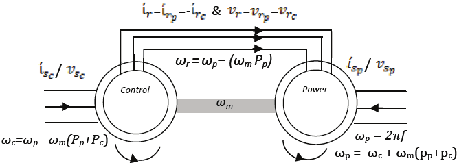
6. The construction for BDFTIG
To establish the complete mathematical representation of the dynamic behaviour of the
BDFTIG it is first necessary to clarify the kind of the electromechanical interconnection that
exists between the cascaded machines. One of the simplest ways to connect these two
machines is in the back-to-back method with no phase inversion on the rotor side, as shown
by Figure 6.
Fig. 6. BDFTIG Back-to-Back Connection
By this connection, the rotor currents produced by the two machines join in the subtractive
style, and the rotor voltages have the same signs, i.e. Irp = −Irc and Vrp = Vrc. The chosen connection really affects the distribution of the magnetic fields and flux inside the BDFTIG,
producing the two counter-rotating torques as will be discussed in the following sections.
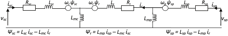
6.1 Equivalent circuit analysis of the BDFTIG
Figure 7- shows the equivalent circuit of the BDFTIG from which the electrical system
equations can be derived.
Fig. 7. Equivalent Circuit of the BDFTIG
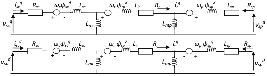
To simplify the controller algorithm, the machine quantities should be expressed in the d-q
frame by employing Park’s and Clark’s transformation. The reason of this transformations is
to remove as many time-varying quantities from the system as possible. By converting the
three-phase machine to its two-phase equivalent and selecting the suitable reference frame,
all the time-varying inductances in both the stator and the rotor are eliminated, allowing for
a simple however complete dynamic model of the electric machine. From these equivalent
circuits the electrical equations of BDFTIG can be determined as shown in the next section.
6.2 Electrical system equations for BDFTIG
Starting with the power machine, the general form of the vector equations of the BDFTIG can
be written as:
q
q
disp
dirp
vqsp
= Rspiqsp + Lsp
+ ω
+ ω
dt
p Lspid
sp + Lmp dt
p Lmpid
r p
q
q
q
q
vsp
= Rspisp + ( Lspisp + Lmpirp) s + ( Lspidsp + Lmpidrp) ωp


From Dynamic Modeling to Experimentation of
Induction Motor Powered by Doubly-Fed Induction Generator by Passivity-Based Control
127
Fig. 8. Equivalent Circuits of d-q BDFTIG
The flux linkage current relations are:
Ψ q
q
q
sp
= Lspisp + Lmpirp
Ψ dsp = Lspidsp + Lmpidrp
(53)
q
q
dΨ qsp
vsp
= Rspisp +
+ ω
dt
pΨ dsp
(54)
q
q
q
q
dirp
disp
vrp
= Rrpirp + Lrp
+ ω
+ ω
dt
r Lr pid
r p + Lmp dt
r Lmpid
sp
q
q
q
q
vrp
= Rrpirp + ( Lrpirp + Lmpisp) s + ( Lrpidrp + Lmpidsp) ωr
We have also:
Ψ qrp = Lrpiqrp + Lmpiqsp
Ψ drp = Lrpidrp + Lmpidsp
(55)
q
q
dΨ qrp
vrp
= Rrpisp +
+ ω
dt
pΨ d
r p
(56)
didsp
q
didrp
q
vdsp = Rspidsp + Lsp
− ω
− ω
dt
p Lspisp + Lmp dt
p Lmpir p
q
q
vdsp = Rspidsp + ( Lspidsp + Lmpidrp) s − ( Lspisp + Lmpirp) ωp dΨ dsp
vdsp = Rspidsp +
− ω
dt
pΨ qsp
(57)
didrp
q
didsp
q
vdrp = Rrpidrp + Lrp
+ ω
+ ω
dt
r Lr pir p + Lmp dt
r Lmpisp
vdrp = Rrpidrp + ( Lrpidrp + Lmpidsp) s + ( Lrpiqrp + Lmpiqsp) ωr dΨ drp
vdrp = Rrpidsp +
+ ω
dt
pΨ qrp
(58)
Electrical system equations for control machine:
q
q
di
di
vq
sc
rc
sc
= Rsciqsc + Lsc
+ ω
+ ω
dt
c Lscid
sc + Lmc dt
c Lmcid
rc
q
q
q
q
vsc
= Rscisc + ( Lscisc + Lmcirc) s + ( Lscidsp + Lmcidrc) ωc


128
Electric Machines and Drives
The flux linkage current relations are:
Ψ qrc = Lsciqsc + Lmciqrc
Ψ dsc = Lscidsp + Lmcidrc
(59)
q
q
vsc
= Rscisc + dΨ qsc + ω
dt
cΨ dsc
(60)
q
q
q
q
di
di
v
rc
sc
rc
= Rrcirc + Lrc
+ ω
+ ω
dt
r Lrcid
rc + Lmc dt
r Lmcid
sc
q
q
q
q
vrc
= Rrcirc + ( Lrcirc + Lmcisc) s + ( Lrpidrp + Lmcidsc) ωr
and:
Ψ q
q
q
rc
= Lrcirc + Lmcisc
Ψ drc = Lrcidrc + Lmcidsc
(61)
q
q
vrc
= Rrcirc + dΨ qrc + ω
dt
r Ψ d
rc
(62)
did
q
did
q
vd
sc
rc
sc
= Rrcidsc + Lsc
− ω
− ω
dt
c Lscisc + Lmc dt
c Lmcirc
q
q
vdsc = Rscidsc + ( Lscidsc + Lmcidrc) s − ( Lscisc + Lmcirc) ωc vdsc = Rscidsc + dΨ dsc − ω
dt
cΨ qsc
(63)
did
q
did
q
vd
rc
sc
rc
= Rrcidrc + Lrc
+ ω
+ ω
dt
c Lrcirc + Lmc dt
r Lmcisc
vdrc = Rrcidrc + ( Lrcidrc + Lmcidsc) s + ( Lrpiqrp + Lmciqsc) ωr vdrc = Rrcidrc + dΨ drc + ω
dt
r Ψ qrc
(64)
As mentioned before, for the BDFTIG with the back-to-back configuration and with no phase
inversion, the rotor currents of the individual machines have the opposite signs, the fluxes
inside the rotor combine to produce the essential ro