Think Stats: Probability and Statistics for Programmers by Allen Downey - HTML preview

Chapter 9

Correlation

9.1

Standard scores

In this chapter we look at relationships between variables. For example, we

have a sense that height is related to weight; people who are taller tend to

be heavier. Correlation is a description of this kind of relationship.

A challenge in measuring correlation is that the variables we want to com-

pare might not be expressed in the same units. For example, height might

be in centimeters and weight in kilograms. And even if they are in the same

units, they come from different distributions.

There are two common solutions to these problems:

1. Transform all values to standard scores. This leads to the Pearson

coefficient of correlation.

2. Transform all values to their percentile ranks. This leads to the Spear-

man coefficient.

If X is a series of values, xi, we can convert to standard scores by subtracting

the mean and dividing by the standard deviation: zi = (xi − µ) / σ.

The numerator is a deviation: the distance from the mean. Dividing by

σ normalizes the deviation, so the values of Z are dimensionless (no units) and their distribution has mean 0 and variance 1.

If X is normally-distributed, so is Z; but if X is skewed or has outliers, so

does Z. In those cases it is more robust to use percentile ranks. If Rcontains

the percentile ranks of the values in X, the distribution of Ris uniform be-

tween 0 and 100, regardless of the distribution of X.

108

Chapter 9. Correlation

9.2

Covariance

Covariance is a measure of the tendency of two variables to vary together.

If we have two series, X and Y, their deviations from the mean are

dxi = xi − µ X

dyi = yi − µ Y

where µ X is the mean of X and µ Y is the mean of Y. If X and Y vary together, their deviations tend to have the same sign.

If we multiply them together, the product is positive when the deviations

have the same sign and negative when they have the opposite sign. So

adding up the products gives a measure of the tendency to vary together.

Covariance is the mean of these products:

1

Cov(X, Y) =

∑ dx

n

idyi

where n is the length of the two series (they have to be the same length).

Covariance is useful in some computations, but it is seldom reported as a

summary statistic because it is hard to interpret. Among other problems, its

units are the product of the units of X and Y. So the covariance of weight

and height might be in units of kilogram-meters, which doesn’t mean much.

Exercise 9.1 Write a function called ❈♦✈ that takes two lists and computes

their covariance. To test your function, compute the covariance of a list

with itself and confirm that Cov(X, X) = Var(X).

You can download a solution from ❤tt♣✿✴✴t❤✐♥❦st❛ts✳❝♦♠✴❝♦rr❡❧❛t✐♦♥✳

♣②.

9.3

Correlation

One solution to this problem is to divide the deviations by σ, which yields

standard scores, and compute the product of standard scores:

(x

(y

p

i − µ X )

i − µ Y )

i =

σ X

σ Y

The mean of these products is

1

ρ =

∑ p

n

i

9.3. Correlation

109

This value is called Pearson’s correlation after Karl Pearson, an influential

early statistician. It is easy to compute and easy to interpret. Because stan-

dard scores are dimensionless, so is ρ.

Also, the result is necessarily between −1 and +1. To see why, we can

rewrite ρ by factoring out σ X and σ Y:

Cov(X, Y)

ρ =

σ X σ Y

Expressed in terms of deviations, we have

∑ dxidyx

ρ = ∑ dxi ∑ dyi

Then by the ever-useful Cauchy-Schwarz inequality1, we can show that

2

ρ ≤ 1, so −1 ≤ ρ ≤ 1.

The magnitude of ρ indicates the strength of the correlation. If ρ = 1 the variables are perfectly correlated, which means that if you know one, you can

make a perfect prediction about the other. The same is also true if ρ = −1.

It means that the variables are negatively correlated, but for purposes of

prediction, a negative correlation is just as good as a positive one.

Most correlation in the real world is not perfect, but it is still useful. For

example, if you know someone’s height, you might be able to guess their

weight. You might not get it exactly right, but your guess will be better

than if you didn’t know the height. Pearson’s correlation is a measure of

how much better.

So if ρ = 0, does that mean there is no relationship between the variables?

Unfortunately, no. Pearson’s correlation only measures linear relationships.

If there’s a nonlinear relationship, ρ understates the strength of the depen-

dence.

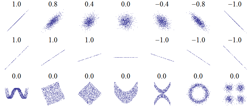
Figure

9.1

is

from

❤tt♣✿✴✴✇✐❦✐♣❡❞✐❛✳♦r❣✴✇✐❦✐✴❈♦rr❡❧❛t✐♦♥❴❛♥❞❴

❞❡♣❡♥❞❡♥❝❡. It shows scatterplots and correlation coefficients for several

carefully-constructed datasets.

The top row shows linear relationships with a range of correlations; you

can use this row to get a sense of what different values of ρ look like.

The second row shows perfect correlations with a range of slopes, which

1See ❤tt♣✿✴✴✇✐❦✐♣❡❞✐❛✳♦r❣✴✇✐❦✐✴❈❛✉❝❤②✲❙❝❤✇❛r③❴✐♥❡q✉❛❧✐t②.

110

Chapter 9. Correlation

Figure 9.1: Examples of datasets with a range of correlations.

demonstrates that correlation is unrelated to slope (we’ll talk about esti-

mating slope soon). The third row shows variables that are clearly related,

but because the relationship is non-linear, the correlation coefficient is 0.

The moral of this story is that you should always look at a scatterplot of

your data before blindly computing a correlation coefficient.

Exercise 9.2 Write a function called ❈♦rr that takes two lists and computes

their correlation. Hint: use t❤✐♥❦st❛ts✳❱❛r and the ❈♦✈ function you wrote

in the previous exercise.

To test your function, compute the covariance of a list with itself and

confirm that Corr(X, X) is 1. You can download a solution from ❤tt♣✿

✴✴t❤✐♥❦st❛ts✳❝♦♠✴❝♦rr❡❧❛t✐♦♥✳♣②.

9.4

Making scatterplots in pyplot

The simplest way to check for a relationship between two variables is a scat-

terplot, but making a good scatterplot is not always easy. As an example, I’ll

plot weight versus height for the respondents in the BRFSS (see Section 4.5).

♣②♣❧♦t provides a function named s❝❛tt❡r that makes scatterplots:

✐♠♣♦rt ♠❛t♣❧♦t❧✐❜✳♣②♣❧♦t ❛s ♣②♣❧♦t

♣②♣❧♦t✳s❝❛tt❡r✭❤❡✐❣❤ts✱ ✇❡✐❣❤ts✮

Figure 9.2 shows the result. Not surprisingly, it looks like there is a positive

correlation: taller people tend to be heavier. But this is not the best represen-

tation of the data, because the data are packed into columns. The problem is

9.4. Making scatterplots in pyplot

111

200

180

160

140

120

100

Weight (kg) 80

60

40

140

20

150

160

170

180

190

200

210

Height (cm)

Figure 9.2: Simple scatterplot of weight versus height for the respondents

in the BRFSS.

200

180

160

140

120

100

Weight (kg) 80

60

40

140

20

150

160

170

180

190

200

210

Height (cm)

Figure 9.3: Scatterplot with jittered data.

112

Chapter 9. Correlation

200

180

160

140

120

100

Weight (kg) 80

60

40

140

20

150

160

170

180

190

200

210

Height (cm)

Figure 9.4: Scatterplot with jittering and transparency.

200

180

160

140

120

100

Weight (kg) 80

60

40

140

20

150

160

170

180

190

200

210

Height (cm)

Figure 9.5: Scatterplot with binned data using ♣②♣❧♦t✳❤❡①❜✐♥.

9.4. Making scatterplots in pyplot

113

that the heights were rounded to the nearest inch, converted to centimeters,

and then rounded again. Some information is lost in translation.

We can’t get that information back, but we can minimize the effect on the

scatterplot by jittering the data, which means adding random noise to re-

verse the effect of rounding off. Since these measurements were rounded to

the nearest inch, they can be off by up to 0.5 inches or 1.3 cm. So I added

uniform noise in the range −1.3 to 1.3:

❥✐tt❡r ❂ ✶✳✸

❤❡✐❣❤ts ❂ ❬❤ ✰ r❛♥❞♦♠✳✉♥✐❢♦r♠✭✲❥✐tt❡r✱ ❥✐tt❡r✮ ❢♦r ❤ ✐♥ ❤❡✐❣❤ts❪

Figure 9.3 shows the result. Jittering the data makes the shape of the re-

lationship clearer. In general you should only jitter data for purposes of

visualization and avoid using jittered data for analysis.

Even with jittering, this is not the best way to represent the data. There are

many overlapping points, which hides data in the dense parts of the figure

and gives disproportionate emphasis to outliers.

We can solve that with the ❛❧♣❤❛ parameter, which makes the points partly

transparent:

♣②♣❧♦t✳s❝❛tt❡r✭❤❡✐❣❤ts✱ ✇❡✐❣❤ts✱ ❛❧♣❤❛❂✵✳✷✮

Figure 9.4 shows the result. Overlapping data points look darker, so dark-

ness is proportional to density. In this version of the plot we can see an

apparent artifact: a horizontal line near 90 kg or 200 pounds. Since this

data is based on self-reports in pounds, the most likely explanation is some

responses were rounded off (possibly down).

Using transparency works well for moderate-sized datasets, but this figure

only shows the first 1000 records in the BRFSS, out of a total of 414509.

To handle larger datasets, one option is a hexbin plot, which divides the

graph into hexagonal bins and colors each bin according to how many data

points fall in it. ♣②♣❧♦t provides a function called ❤❡①❜✐♥:

♣②♣❧♦t✳❤❡①❜✐♥✭❤❡✐❣❤ts✱ ✇❡✐❣❤ts✱ ❝♠❛♣❂♠❛t♣❧♦t❧✐❜✳❝♠✳❇❧✉❡s✮

Figure 9.5 shows the result with a blue colormap. An advantage of a hexbin

is that it shows the shape of the relationship well, and it is efficient for large

datasets. A drawback is that it makes the outliers invisible.

The moral of this story is that it is not easy to make a scatterplot that is not

potentially misleading. You can download the code for these figures from

❤tt♣✿✴✴t❤✐♥❦st❛ts✳❝♦♠✴❜r❢ss❴s❝❛tt❡r✳♣②.

114

Chapter 9. Correlation

9.5

Spearman’s rank correlation

Pearson’s correlation works well if the relationship between variables is lin-

ear and if the variables are roughly normal. But it is not robust in the pres-

ence of outliers.

Anscombe’s quartet demonstrates this effect; it contains four data sets with

the same correlation. One is a linear relation with random noise, one is a

non-linear relation, one is a perfect relation with an outlier, and one has no

relation except an artifact caused by an outlier. You can read more about it

at ❤tt♣✿✴✴✇✐❦✐♣❡❞✐❛✳♦r❣✴✇✐❦✐✴❆♥s❝♦♠❜❡✬s❴q✉❛rt❡t.

Spearman’s rank correlation is an alternative that mitigates the effect of out-

liers and skewed distributions. To compute Spearman’s correlation, we

have to compute the rank of each value, which is its index in the sorted

sample. For example, in the sample {7, 1, 2, 5} the rank of the value 5 is 3,

because it appears third if we sort the elements. Then we compute Pearson’s

correlation for the ranks.

An alternative to Spearman’s is to apply a transform that makes the data

more nearly normal, then compute Pearson’s correlation for the trans-

formed data. For example, if the data are approximately lognormal, you

could take the log of each value and compute the correlation of the logs.

Exercise 9.3 Write a function that takes a sequence and returns a list that

contains the rank for each element. For example, if the sequence is {7, 1, 2,

5}, the result should be { 4, 1, 2, 3}.

If the same value appears more than once, the strictly correct solution is to

assign each of them the average of their ranks. But if you ignore that and

assign them ranks in arbitrary order, the error is usually small.

Write a function that takes two sequences (with the same length) and com-

putes their Spearman rank coefficient. You can download a solution from

❤tt♣✿✴✴t❤✐♥❦st❛ts✳❝♦♠✴❝♦rr❡❧❛t✐♦♥✳♣②.

Exercise 9.4 Download ❤tt♣✿✴✴t❤✐♥❦st❛ts✳❝♦♠✴❜r❢ss✳♣② and ❤tt♣✿✴✴

t❤✐♥❦st❛ts✳❝♦♠✴❜r❢ss❴s❝❛tt❡r✳♣②. Run them and confirm that you can

read the BRFSS data and generate scatterplots.

Comparing the scatterplots to Figure 9.1, what value do you expect for Pear-

son’s correlation? What value do you get?

Because the distribution of adult weight is lognormal, there are outliers that

affect the correlation. Try plotting log(weight) versus height, and compute

Pearson’s correlation for the transformed variable.

9.6. Least squares fit

115

Finally, compute Spearman’s rank correlation for weight and height. Which

coefficient do you think is the best measure of the strength of the relation-

ship? You can download a solution from ❤tt♣✿✴✴t❤✐♥❦st❛ts✳❝♦♠✴❜r❢ss❴

❝♦rr✳♣②.

9.6

Least squares fit

Correlation coefficients measure the strength and sign of a relationship, but

not the slope. There are several ways to estimate the slope; the most com-

mon is a linear least squares fit. A “linear fit” is a line intended to model the

relationship between variables. A “least squares” fit is one that minimizes

the mean squared error (MSE) between the line and the data2.

Suppose we have a sequence of points, Y, that we want to express as a

function of another sequence X. If there is a linear relationship between

X and Y with intercept α and slope β, we expect each yi to be roughly α +

β xi.

But unless the correlation is perfect, this prediction is only approximate.

The deviation, or residual, is

ε i = ( α + β xi) − yi

The residual might be due to random factors like measurement error, or

non-random factors that are unknown. For example, if we are trying to

predict weight as a function of height, unknown factors might include diet,

exercise, and body type.

If we get the parameters α and β wrong, the residuals get bigger, so it makes intuitive sense that the parameters we want are the ones that minimize the

residuals.

As usual, we could minimize the absolute value of the residuals, or their

squares, or their cubes, etc. The most common choice is to minimize the

sum of squared residuals

min ∑ 2

ε i

α, β

Why? There are three good reasons and one bad one:

• Squaring has the obvious feature of treating positive and negative

residuals the same, which is usually what we want.

2See ❤tt♣✿✴✴✇✐❦✐♣❡❞✐❛✳♦r❣✴✇✐❦✐✴❙✐♠♣❧❡❴❧✐♥❡❛r❴r❡❣r❡ss✐♦♥.

116

Chapter 9. Correlation

• Squaring gives more weight to large residuals, but not so much weight

that the largest residual always dominates.

• If the residuals are independent of x, random, and normally dis-

tributed with µ = 0 and constant (but unknown) σ, then the least

squares fit is also the maximum likelihood estimator of α and β.3

• The values of ˆ α and ˆ β that minimize the squared residuals can be computed efficiently.

That last reason made sense when computational efficiency was more im-

portant than choosing the method most appropriate to the problem at hand.

That’s no longer the case, so it is worth considering whether squared resid-

uals are the right thing to minimize.

For example, if you are using values of X to predict values of Y, guessing

too high might be better (or worse) than guessing too low. In that case you

might want to compute some cost function, cost( ε i), and minimize total cost.

However, computing a least squares fit is quick, easy and often good

enough, so here’s how:

1. Compute the sample means, ¯x and ¯y, the variance of X, and the co-

variance of X and Y.

2. The estimated slope is

ˆ

Cov(X, Y)

β =

Var(X)

3. And the intercept is

ˆ α = ¯y − ˆ β ¯x

To see how this is derived, you can read ❤tt♣✿✴✴✇✐❦✐♣❡❞✐❛✳♦r❣✴✇✐❦✐✴

◆✉♠❡r✐❝❛❧❴♠❡t❤♦❞s❴❢♦r❴❧✐♥❡❛r❴❧❡❛st❴sq✉❛r❡s.

Exercise 9.5 Write a function named ▲❡❛st❙q✉❛r❡s that takes X and Y and

computes ˆ α and ˆ β. You can download a solution from ❤tt♣✿✴✴t❤✐♥❦st❛ts✳

❝♦♠✴❝♦rr❡❧❛t✐♦♥✳♣②.

Exercise 9.6 Using the data from the BRFSS again, compute the linear least

squares fit for log(weight) versus height. You can download a solution from

❤tt♣✿✴✴t❤✐♥❦st❛ts✳❝♦♠✴❜r❢ss❴❝♦rr✳♣②.

3See Press et al., Numerical Recipes in C, Chapter 15 at ❤tt♣✿✴✴✇✇✇✳♥r❜♦♦❦✳❝♦♠✴❛✴

❜♦♦❦❝♣❞❢✴❝✶✺✲✶✳♣❞❢.

9.7. Goodness of fit

117

Exercise 9.7 The distribution of wind speeds in a given location deter-

mines the wind power density, which is an upper bound on the aver-

age power that a wind turbine at that location can generate. According

to some sources, empirical distributions of wind speed are well modeled

by a Weibull distribution (see ❤tt♣✿✴✴✇✐❦✐♣❡❞✐❛✳♦r❣✴✇✐❦✐✴❲✐♥❞❴♣♦✇❡r★

❉✐str✐❜✉t✐♦♥❴♦❢❴✇✐♥❞❴s♣❡❡❞).

To evaluate whether a location is a viable site for a wind turbine, you can

set up an anemometer to measure wind speed for a period of time. But it is

hard to measure the tail of the wind speed distribution accurately because,

by definition, events in the tail don’t happen very often.

One way to address this problem is to use measurements to estimate the

parameters of a Weibull distribution, then integrate over the continuous

PDF to compute wind power density.

To estimate the parameters of a Weibull distribution, we can use the trans-

formation from Exercise 4.6 and then use a linear fit to find the slope and

intercept of the transformed data.

Write a function that takes a sample from a Weibull distribution and esti-

mates its parameters.

Now write a function that takes the parameters of a Weibull distribution of

wind speed and computes average wind power density (you might have to

do some research for this part).

9.7

Goodness of fit

Having fit a linear model to the data, we might want to know how good it

is. Well, that depends on what it’s for. One way to evaluate a model is its

predictive power.

In the context of prediction, the quantity we are trying to guess is called

a dependent variable and the quantity we are using to make the guess is

called an explanatory or independent variable.

To measure the predictive power of a model, we can compute the coefficient

of determination, more commonly known as “R-squared”:

Var( ε)

R2 = 1 − Var(Y)

118

Chapter 9. Correlation

To understand what R2 means, suppose (again) that you are trying to guess

someone’s weight. If you didn’t know anything about them, your best strat-

egy would be to guess ¯y; in that case the MSE of your guesses would be

Var(Y):

1

MSE =

∑( ¯y − y

n

i)2 = Var(Y)

But if I told you their height, you would guess ˆ α + ˆ β xi; in that case your MSE would be Var( ε).

1

MSE =

∑(ˆ α + ˆ β x

n

i − yi)2 = Var( ε)

So the term Var( ε)/Var(Y) is the ratio of mean squared error with and with-

out the explanatory variable, which is the fraction of variability left unex-

plained by the model. The complement, R2