not stochastically independent. To see this, assume the first letter to be "b", then it is more
probable that the next letter is "e", than "z". In the case where the outcomes are not
stochastically independent, the formulation we have given of Shannon's source coding
theorem is no longer valid, to fix this, we should replace the entropy with the entropy rate, but
we will not pursue this here).
Generating efficient codes
From Shannon's source coding theorem we know what the minimum average rate needed to
represent a source is. But other than in the case when the logarithm of the probabilities gives an
integer, we do not get any indications on how to obtain that rate. It is a large area of research to
get close to the Shannon entropy bound. One clever way to do encoding is the Huffman coding
scheme.
5.4. Entropy*
The self information gives the information in a single outcome. In most cases, e.g in data compression, it is much more interesting to know the average information content of a source.
This average is given by the expected value of the self information with respect to the source's
probability distribution. This average of self information is called the source entropy.
Definition of entropy
Definition: Entropy
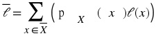
1. The entropy (average self information) of a discrete random variable X is a function of its
probability mass function and is defined as
(5.1)
where N is the number of possible values of X and P X ( x i ) = Pr[ X = x i ] . If log is base 2 then the unit of entropy is bits per (source)symbol. Entropy is a measure of uncertainty in a random
variable and a measure of information it can reveal.
2. If symbol has zero probability, which means it never occurs, it should not affect the entropy.
Letting 0log0 = 0 , we have dealt with that.
In texts you will find that the argument to the entropy function may vary. The two most common
are H( X) and H( p) . We calculate the entropy of a source X, but the entropy is, strictly speaking, a function of the source's probabilty function p. So both notations are justified.
Calculating the binary logarithm
Most calculators does not allow you to directly calculate the logarithm with base 2, so we have to
use a logarithm base that most calculators support. Fortunately it is easy to convert between
different bases.
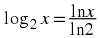
Assume you want to calculate log2 x , where x > 0 . Then log2 x = y implies that 2 y = x . Taking the natural logarithm on both sides we obtain
Logarithm conversion
Examples
Example 5.7.
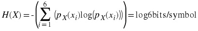
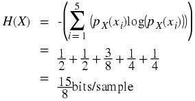
When throwing a dice, one may ask for the average information conveyed in a single throw.
Using the formula for entropy we get
Example 5.8.
If a soure produces binary information {0, 1} with probabilities p and 1 − p . The entropy of
the source is H( X) = – ( p log2 p) − (1 − p)log2(1 − p) If p = 0 then H( X) = 0 , if p = 1 then H( X) = 0 , if p = 1 / 2 then H( X) = 1 . The source has its largest entropy if p = 1 / 2 and the source provides no new information if p = 0 or p = 1 .
Figure 5.3.


Example 5.9.
An analog source is modeled as a continuous-time random process with power spectral density
bandlimited to the band between 0 and 4000 Hz. The signal is sampled at the Nyquist rate. The
sequence of random variables, as a result of sampling, are assumed to be independent. The
samples are quantized to 5 levels {-2, -1, 0, 1, 2} . The probability of the samples taking the
quantized values are
, respectively. The entropy of the random variables are
There are 8000 samples per second. Therefore, the source produces
bits/sec of information.
Entropy is closely tied to source coding. The extent to which a source can be compressed is related
to its entropy. There are many interpretations possible for the entropy of a random variable,
including
(Average)Self information in a random variable
Minimum number of bits per source symbol required to describe the random variable without
loss
Description complexity
Measure of uncertainty in a random variable
References
Øien, G.E. and Lundheim,L. (2003) Information Theory, Coding and Compression,

Trondheim: Tapir Akademisk forlag.
5.5. Differential Entropy*
Consider the entropy of continuous random variables. Whereas the (normal) entropy is the entropy of a discrete random variable, the differential entropy is the entropy of a continuous
random variable.
Differential Entropy
Definition: Differential entropy
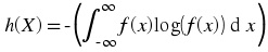
The differential entropy h( X) of a continuous random variable X with a pdf f( x) is defined as Usually the logarithm is taken to be base 2, so that the unit of the differential entropy is
bits/symbol. Note that is the discrete case, h( X) depends only on the pdf of X . Finally, we note that the differential entropy is the expected value of – (log( f( x))) , i.e., h( X) = – ( E(log( f( x)))) Now, consider a calculating the differential entropy of some random variables.
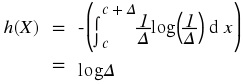
Example 5.10.
Consider a uniformly distributed random variable X from c to c + Δ . Then its density is from c to c + Δ , and zero otherwise.
We can then find its differential entropy as follows,
Note that by making
Δ arbitrarily small, the differential entropy can be made arbitrarily negative, while taking
Δ arbitrarily large, the differential entropy becomes arbitrarily positive.
Example 5.11.
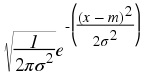
Consider a normal distributed random variable X , with mean m and variance σ 2 . Then its
density is
.
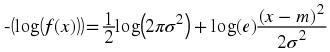
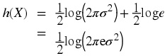
We can then find its differential entropy as follows, first calculate – (log( f( x))):
Then since E(( X − m)2) = σ 2 , we have


Properties of the differential entropy
In the section we list some properties of the differential entropy.
The differential entropy can be negative
h( X + c) = h( X) , that is translation does not change the differential entropy.
h( aX) = h( X) + log(| a|) , that is scaling does change the differential entropy.
The first property is seen from both Example 5.10 and Example 5.11. The two latter can be shown by using Equation.
5.6. Huffman Coding*
One particular source coding algorithm is the Huffman encoding algorithm. It is a source coding algorithm which approaches, and sometimes achieves, Shannon's bound for source compression. A
brief discussion of the algorithm is also given in another module.
Huffman encoding algorithm
1. Sort source outputs in decreasing order of their probabilities
2. Merge the two least-probable outputs into a single output whose probability is the sum of the
corresponding probabilities.
3. If the number of remaining outputs is more than 2, then go to step 1.
4. Arbitrarily assign 0 and 1 as codewords for the two remaining outputs.
5. If an output is the result of the merger of two outputs in a preceding step, append the current
codeword with a 0 and a 1 to obtain the codeword the the preceding outputs and repeat step 5.
If no output is preceded by another output in a preceding step, then stop.
Example 5.12.
X ∈ { A, B, C, D} with probabilities { , , , }
Figure 5.4.


. As you may recall, the entropy of the source was also
.
In this case, the Huffman code achieves the lower bound of
.
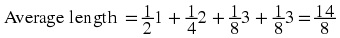
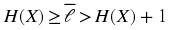
In general, we can define average code length as
where is the set of possible
values of x .
It is not very hard to show that
For compressing single source output at a time,
Huffman codes provide nearly optimum code lengths.
The drawbacks of Huffman coding
1. Codes are variable length.
2. The algorithm requires the knowledge of the probabilities, p X ( x) for all
.
Another powerful source coder that does not have the above shortcomings is Lempel and Ziv.
Chapter 6. Decibel scale with signal processing
applications*
6.1. Introduction
The concept of decibel originates from telephone engineers who were working with power loss in
a telephone line consisting of cascaded circuits. The power loss in each circuit is the ratio of the
power in to the power out, or equivivalently, the power gain is the ratio of the power out to the
power in.
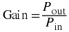
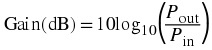
Let P in be the power input to a telephone line and P out the power out. The power gain is then
given by
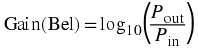
Taking the logarithm of the gain formula we obtain a comparative measure
called Bel.
Bel
This measure is in honour of Alexander G. Bell, see Figure 6.1.
Figure 6.1.
Alexander G. Bell
6.2. Decibel
Bel is often a to large quantity, so we define a more useful measure, decibel:
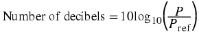

Please note from the definition that the gain in dB is relative to the input power. In general we
define:
If no reference level is given it is customary to use P ref = 1 W , in which case we have:
Decibel
Number of decibels = 10log10( P)
Example 6.1.
Given the power spectrum density (psd) function of a signal x( n), S xx( ⅈf) . Express the magnitude of the psd in decibels.
We find S xx(dB) = 10log10(| S xx( ⅈf)|) .
6.3. More about decibels
Above we’ve calculated the decibel equivalent of power. Power is a quadratic variable, whereas
voltage and current are linear variables. This can be seen, for example, from the formulas
and P = I 2 R .
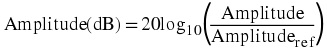
So if we want to find the decibel value of a current or voltage, or more general an amplitude we
use:
This is illustrated in the following example.
Example 6.2.
Express the magnitude of the filter H( ⅈf) in dB scale.
The magnitude is given by | H( ⅈf)| , which gives: | H(dB)| = 20log10(| H( ⅈf)|) .
Plots of the magnitude of an example filter | H( ⅈf)| and its decibel equivalent are shown in
Figure 6.2.
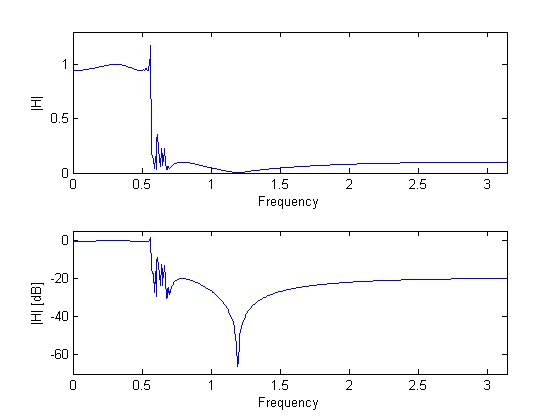
Magnitude responses.
6.4. Some basic arithmetic
The ratios 1,10,100, 1000 give dB values 0 dB, 10 dB, 20 dB and 30 dB respectively. This implies
that an increase of 10 dB corresponds to a ratio increase by a factor 10.
This can easily be shown: Given a ratio R we have R[dB] = 10 log R. Increasing the ratio by a
factor of 10 we have: 10 log (10*R) = 10 log 10 + 10 log R = 10 dB + R dB.
Another important dB-value is 3dB. This comes from the fact that:
An increase by a factor 2 gives: an increase of 10 log 2 ≈ 3 dB. A “increase” by a factor 1/2 gives:
an “increase” of 10 log 1/2 ≈ -3 dB.
Example 6.3.
In filter terminology the cut-off frequency is a term that often appears. The cutoff frequency
(for lowpass and highpass filters), f c , is the frequency at which the squared magnitude response in dB is ½. In decibel scale this corresponds to about -3 dB.
6.5. Decibels in linear systems
In signal processing we have the following relations for linear systems: Y( ⅈf) = H( ⅈf) X( ⅈf) where X and H denotes the input signal and the filter respectively. Taking absolute values on both sides
of Equation and converting to decibels we get:
Input and output relations for linear systems
The output amplitude at a given frequency is simply given by the sum of the filter
gain and the input amplitude, both in dB.
6.6. Other references:
Above we have used P ref = 1 W as a reference and obtained the standard dB measure. In some
applications it is more useful to use P ref = 1 mW and we then have the dBm measure.
Another example is when calculating the gain of different antennas. Then it is customary to use an
isotropic (equal radiation in all directions) antenna as a reference. So for a given antenna we can
use the dBi measure. (i -> isotropic)
6.7. Matlab files
Chapter 7. Filter types*
So what is a filter? In general a filter is a device that discriminates, according to one or more
attributes at its input, what passes through it. One example is the colour filter which absorbs light
at certain wavelengths. Here we shall describe frequency-selective filters. It is called freqency-
selective because it discriminates among the various frequency compononents of its input. By
filter design we can create filters that pass signals with frequency components in some bands, and
attenuates signals with content in other frequency bands.
It is customary to classify filters according to their frequency domain charachteristics. In the
following we will take a look at: lowpass, highpass, bandpass, bandstop, allpass and notch filters.
(All of the filters shown are discrete-time)
7.1. Ideal filter types
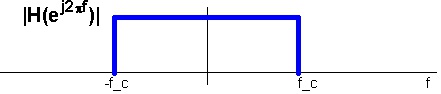
Lowpass
Attenuates frequencies above cutoff frequency, letting frequencies below cutoff( f c ) through, see
Figure 7.1.
An ideal lowpass filter.
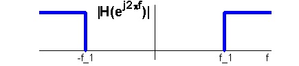
Highpass
Highpass filters stops low frequencies, letting higher frequencies through, see Figure 7.2.
Figure 7.2.
An ideal highpass filter.
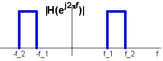
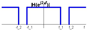
Bandpass
Letting through only frequencies in a certain range, see Figure 7.3.
Figure 7.3.
An ideal bandpass filter.
Bandstop
Stopping frequencies in a certain range, see Figure 7.4.
Figure 7.4.
An ideal bandstop filter.
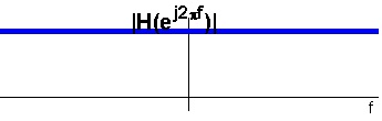
Allpass
Letting all frequencies through, see see Figure 7.5.
Figure 7.5.
An ideal allpass filter.
Does this imply that the allpass filter is useless? The answer is no, because it may have effect on
the signals phase. A filter is allpass if | H( ⅇ ⅈ 2 π f )| = 1 , . The allpass filter finds further applications as building blocks for many higher order filters.
7.2. Other filter types
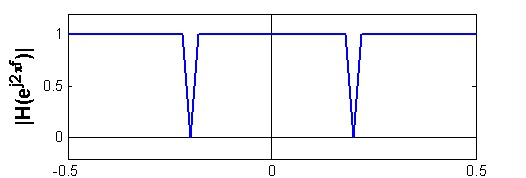
Notch filter
The notch filter recognized by its perfect nulls in the frequency response, see Figure 7.6.
Figure 7.6.
Notch filter.
Notch filters have many applications. One of them is in recording systems, where the notch filter
serve to remove the power-line frequency 50 Hz and its harmonics(100 Hz, 150 Hz,...). Some
audio equalisers include a notch filter.
7.3. Matlab files
Chapter 8. Table of Formulas*
Table 8.1.
Analog
Time Discrete
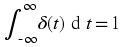
Delta function
Unit sample
δ( t) = 0 for t ≠ 0,
Unit step function
Unit step function
Angular frequency
Angular frequency
Ω = 2 π F
ω = 2 π f
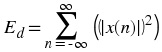
Energy
Energy
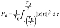
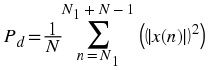
Power
Power
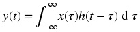
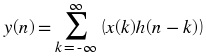
Convol.
Convol.
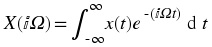
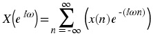
Fourier Transformation
Discrete Time Fourier Transform
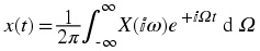
Inverse Fourier Transform
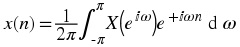
Inverse DTFT