ANIMAL ECOLOGY
Estimation of dissolved oxygen (DO) content in the given water sample by Winkler’s method.
Theory: Dissolved oxygen (DO) determination quantifies the amount of dissolved (or free) oxygen available in water. Aquatic organisms such as fish, crustaceans, mollusks and aerobic bacteria need dissolved oxygen to survive. When dissolve oxygen level in water reduces, the environment becomes less capable of sustaining living forms and even aerobic bacteria which are involved in the decomposition of sewage waste do not survive. The concentration of dissolved oxygen can be easily and accurately determined by the method of Winkler (1888).
Principle: Dissolved oxygen in water doesn’t reacts with KI directly; therefore manganese hydroxide is used as an oxygen carrier. Mn(OH)2 (manganese hydroxide) is produced by the reaction of KOH with MnSO4. Mn(OH)2 reacts with dissolved molecular oxygen to form a brown colored precipitate of MnO(OH)2 (manganic oxide). This manganic oxide then reacts with concentrated sulphuric acid to liberate nascent oxygen, which results in oxidation of KI to I2. This liberated iodine is then titrated against standard sodium thiosulphate solution using starch as an indicator. Thiosulphate reduces iodine to iodide ions and itself gets oxidized to tetrathionate ion.
Reactions:
2KOH + MnSO4 =Mn(OH)2 + K2SO4
2Mn (OH)2 + O2 =2MnO (OH)2
MnO (OH)2 + H2SO4 =MnSO4 + 2H2O + [O]
2KI + H2SO4 + [O] =K2SO4 + H2O + I2
2S2O 3 2- + I2= S4O 62- + 2I-
Chemical preparation:
Procedure:
Calculate dissolve oxygen as follows:
When the whole contents have been titrated:
When only a part of content has been titrated:
Where, 0.2 value represents, 1ml of sodium thiosulphate equivalent to 0.2 mg of O2
Estimation of water alkalinity from given water sample.
Theory: Alkalinity of water is the measure of acid-neutralizing or buffering capacity of water. Alkalinity in water is due to the presence of bicarbonate, carbonate, and hydroxide ions, which provides buffering capacity to water. Buffering capacity works by absorbing positively charged hydrogen ions by using negatively charged bicarbonate and carbonate molecules, which resist any substantial change in the pH. Therefore, a water sample with high alkalinity will have more resistance towards any change in pH.Generally acids are added to the water from rain, snow or though soil sources whereas, alkalinity increases as water dissolves rocks containing calcium carbonate such as calcite and limestone.
Alkaninity of water is important for the aquatic species as alkalinity helps in maintaining the pH of water. Generally alkalinity is buffered but acid shock may occur in spring when acid snows melt, thunderstorms or acid rain enter the stream. If increasing amounts of acids are added to a body of water, the water's buffering capacity is all used up. Sensitive species and young one’s are to be affected first though this impact grows further with the food chain as when food species disappear, even bigger and resistant species are affected.The safe limit of alkalinity for sustaining aquatic life should be at least 20 mg/L.
Principle: There are five possible conditions of alkalinity carbonate, bicarbonates, hydroxide ion, carbonate + hydroxide, carbonate + bicarbonate. Alkalinity is determined by titrating the water sample with strong acid.
Requirements: Burette, conical flasks, beakers, weighing balance, measuring cylinder.
Reagents:
1. Phenolphthalein indicator solution:
Dissolve 0.5g phenolphthalein in 50 ml of ethyl alcohol and add 50 ml of distilled water. Add 0.02N NaOH drop wise until a faint pink color appears.
2. Standard sulphuric acid: (0.02N): prepare stock solution, 0.1N by diluting 3 ml of conc. H2SO4 to 1 L. Dilute 200ml of 0.1N stock solution to 2000ml with carbon dioxide free water to give 0.02N solution. This must be standardized against Na2CO3
3. Methyl orange indicator solution: Dissolve 0.5g methyl orange in 2 liters of distilled water.
4. Procedure:
Phenolphthalein alkalinity: Take 50 /100ml of water sample and four drops of phenolphthalein indicator solution. If a pink color appears (indicates the presence of carbonate) titrate against standard H2SO4 (0.02N) until color disappears. pH 8.3 and record ml of acid used.
Total alkalinity: (by methyl orange indicator method)
If no pink color appears after adding phenolphthalein or after phenolphthalein titration, add two drops of methyl orange indicator and titrate to a faint orange at pH 4.6 (and pink at below4 pH). Record total used standard acid in ml.
Calculations:
Study of animal community structure, determination of density, frequency and abundance of species by quadrat method.
Quadrat Sampling in Population Ecology
Background
Estimating the abundance of organisms.
Ecology is often referred to as the "study of distribution and abundance". This being true, we would often like to know how many of a certain organism are in a certain place, or at a certain time. Information on the abundance of an organism, or group of organisms is fundamental to most questions in ecology. However, we can rarely do a complete census of the organisms in the area of interest because of limitations to time or research funds. Therefore, we usually have to estimate the abundance of organisms by sampling them, or counting a subset of the population of interest.
For example, suppose you wanted to know how many snails there were in the forests. It would take a lifetime to count them all, but you could estimate their abundance by counting all the snails in carefully chosen smaller areas on the forest.
Accuracy vs. Precision.
Obviously, we would like our method for sampling the population to produce a good estimate. A "good "estimate should maximize both precision and accuracy. Accuracy refers to how close to the true mean (μ) our estimate is. That is, if we somehow could know the true number of snails residing on forest, we could compare our estimate to it and find out how accurate we are. Obviously, we would like our estimate to be as close to the true value as possible. In addition, we would like to avoid any bias in our estimate. An estimate would be biased if it consistently over- or under-estimated the true mean. Bias may arise in many ways, but one frequent source is by the selection of sample plots that are nonrandom with respect to the abundance of the target organism. For example, if we looked for snails at forest only in sunny, dry open fields, our estimate would probably be much lower than the true abundance. Random sampling avoids this source of bias. A random sample is one where every potential sample plot within the study area sample has an exactly equal chance of being chosen for sampling. Random sampling is not the same as haphazard sampling. True random sampling usually requires the use a random number table, or a random number generator. In addition to obtaining an accurate, unbiased sample, we are also concerned with the precision of our estimates. Precision refers to the repeatability of our estimates of the true sample mean. If we were to estimate snail abundance many times and got nearly the same estimate each time, we would say that our estimate was very precise. Note that it is possible to have accuracy without precision and vice versa.
Some of the factors that affect precision are:
1) Measurement error. In the real world, it is important to count organisms carefully and lay out plots accurately for good estimates of density. This is not a concern here however, because the computer will be laying out the plots and counting the plants.
2) Total area sampled. In general, the more are a sampled, the more precise the estimates will be, but at the expense of additional sampling effort.
3) Dispersion of the population. Whether the population tends to be aggregated, evenly spaced, or randomly dispersed can affect precision. Note that the dispersion pattern of the same population may be different at different spatial scales (e.g., 1 x1 m plots vs 100 x 100 m plots).
4) Size and shape of quadrates. The size and shape of the plots can affect sampling precision. Often, the optimal plot size and shape will depend on the dispersion pattern of the population.
Various experiments protocols for Community Structure Study:
1. Aim of the Experiment:
To determine the minimum size of the quadrat by species area-curve method.
Requirements:
Nails, cord or string, meter scale, hammer, pencil, notebook.
Method:
i. Prepare a L-shaped structure of 1 × 1 meter size in the given area by using 3 nails and tying them with a cord or string.
ii. Measure 10 cm on one side of the arm L and the same on the other side of L, and prepare 10 x 10 sq. cm area using another set of nails and string. Note the number of species in this area of 10 x 10 sq. cm.
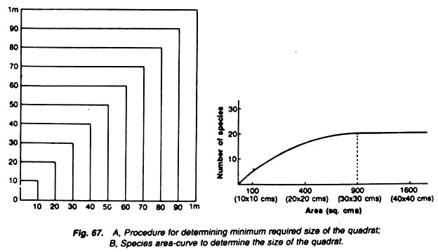
Fig. A. Procedure for determining minimum required size of the quadrate.
B. Species area curve to determine the size of the quadrate.
iii. Increase this area to 20 × 20 sq. cm and note the additional species growing in this area.
iv. Repeat the same procedure for 30 × 30 sq. cm, 40 × 40 sq. cm and so on till 1 × 1 sq. metre area is covered (Fig. 67) and note the number of additional species every time.
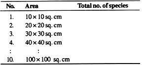
Record your data in the following table:
v. Prepare a graph using the data recorded in the above table. Size of the quadrates is plotted on X- axis and the number of species on Y-axis (Fig. B).
Observations:
The curve starts flattening or shows only a steady increase (Fig. B) at one point in the graph.
Results:
The point of the graph, at which the curve starts flattening or shows only a steady or gradual increase, indicates the minimum size or minimum area of the quadrate suitable for study.
2. Aim of the Experiment:
To study communities by quadrate method and to determine % Frequency, Density and Abundance.
Requirements:
Meter scale, string, four nails or quadrate, notebook.
(i) Frequency:
Frequency is the number of sampling units or quadrates in which a given species occurs.
Percentage frequency (%F) can be estimated by the following formula:

(ii) Density:
Density is the number of individuals per unit area and can be calculated by the following formula:

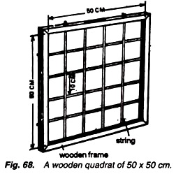
Fig. A wooden quadrate of 50 x 50 cm
(iii) Abundance:
Abundance is described as the number of individuals per quadrate of occurrence.
Abundance for each species can be calculated by the following formula:

Method:
Lay a quadrate (Fig. 68) in the field or specific area to be studied. Note carefully the plants occurring there. Write the names and number of individuals of plant species in the note-book, which are present in the limits of your quadrate. Lay at random at least 10 quadrates (Fig. 69) in the same way and record your data in the form of Table 1.
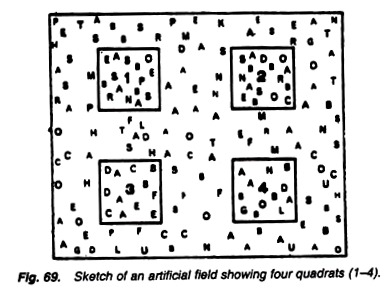
Fig. Sketch of an artificial field showing four quadrates (1-4)
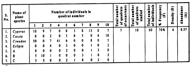
In Table,1 % frequency, density and abundance of Cyperus have been determined. Readings of the other six plants, occurred in the quadrates studied, are also filled in the table. Calculate the frequency, density, and abundance of these six plants for practice. (For the practical class take your own readings. The readings in Table 1 are only to explain the matter).
Observations:
See Table 1
Results:
Calculate the frequency, density, and abundance of all the plant species with the help of the formulae given earlier and note the following results:
(i) In terms of % Frequency (F), the field is being dominated by…
(ii) In terms of Density (D), the field is being dominated by…
(iii) In terms of Abundance (A), the field is being dominated by…
Observations:
Table 1: Size of quadrate: 50cm × 50cm = 2500 cm2
3. Aim of the Experiment:
To determine minimum number of quadrates required for reliable estimate of biomass in grasslands.
Requirements:
Meter scale, string, four nails (or quadrate), note book, graph paper, herbarium sheet, cello tape.
Method:
i. Lay down 20-50 quadrates of definite size at random in the grassland to be studied, make a list of different plant species (e.g., A-J) present in each quadrate and note down their botanical names or hypothetic numbers (e.g., A, B, C,…, J) as shown in Table 2.
ii. With the help of the data available in Table 2, find out the accumulating total of the number of species for each quadrate.
Table 2:showing the accumulating total of the number of species for each quadrat.
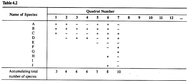
iii. Now take a graph paper sheet and plot the number of quadrates on X-axis and the accumulating total number of species on Y-axis of the graph paper.
Observations and results:
A curve would be obtained. Note carefully that this curve also starts flattening. The point at which this curve starts flattening up would give us the minimum number of quadrats required to be laid down in the grassland.
4. Aim of the Experiment:
To study frequency of herbaceous species in grassland and to compare the frequency distribution with Raunkiaer’s standard frequency diagram.
Requirements:
Quadrat, pencil, note-book, graph paper.
Method:
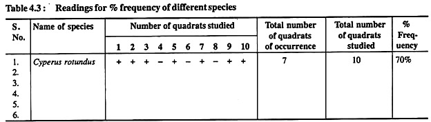
i. Lay 10 quadrats in the given area and calculate the percentage frequency of different plant species by the method and formula given above in Exercise No. 2.
ii. Arrange your data in the form of following Table 3:
Table 3: reading for % frequency of different species
Raunkiaer (1934) classified the species in a community into following five classes as shown in Table 4.4:
Table 4. Classes of species in a community according to Raunkiaer (1934).
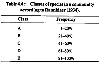
Arrange percentage frequency of different species of the above Table.3 in the five frequency classes (A-E) as formulated by Raunkiaer (1934) in Table 4.
Draw a histogram (Fig.) with the percentage of total number of species plotted on Y-axis and the frequency classes (A-E) on X-axis.
This is the frequency diagram (Fig):
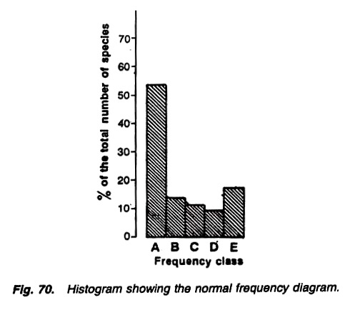
Fig. Histogram showing the normal frequency diagram
Observations and results:
The histogram takes a “J- shaped” curve as suggested by Raunkiaer (1934), and this shows the normal distribution of frequency percentage. If the vegetation in the area is uniform, class ‘E’ is always larger than class ‘D’. And in case class ‘E’ is smaller than class ‘D, the community or vegetation in the area shows considerable disturbance.
5. Aim of the Experiment:
To estimate Importance Value Index for grassland species on the basis of relative frequency, relative density and relative dominance in protected and grazed grassland.
Requirements:
Wooden quadrate of 1×1 meter, pencil, notebook.
What is Importance Value Index?
The Importance Value Index (IVI) shows the complete or overall picture of ecological importance of the species in a community. Community structure study is made by studying frequency, density, abundance, and basal cover of species. But these data do not provide an overall picture of importance of a species, e.g., frequency gives us an idea about dispersion of a species in the area but does not give any idea about its number or the area covered.
Density gives the numerical strength and nothing about the spread or cover. A total picture of the ecological importance of a species in a community is obtained by IVI. For finding IVI, the percentage values of relative frequency, relative density, and relative dominance are added together, and this value out of 300 is called Importance Value Index or IVI of a species.
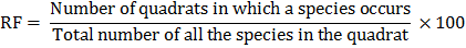
Relative frequency (RF) of a species is calculated by the following formula:
Relative density (RD) of a species is calculated by the following formula:
![]()
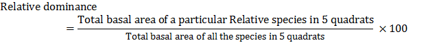
Relative dominance of a species is calculated by the following formula:
Basal area of a plant species is calculated by the following formula:
Basals area of a species = p r2
where p = 3.142, and r = radius of the stem
Method:
i. Find out the values of relative frequency, relative density and relative dominance by the above-mentioned formulae.
ii. Calculate the IVI by adding these three values:
IVI = relative frequency + relative density + relative dominance.
Results:
Arrange the species in order of decreasing importance, i.e., the species having highest IVI is of most ecological importance and the one having the lowest IVI is of least ecological importance.
6. Aim of the Experiment:
To determine the basal cover, or vegetational cover of one herbaceous community by quadrate method.
Requirements:
Wooden quadrate of 1×1 m, Vernier-calliper, pencil, notebook.
Method:
i. Lay a wooden-framed quadrate of 1 x 1 meter randomly in a selected plot of vegetation and count the total number of individuals of the selected species inside the quadrate.
ii. Cut a few stems of some plants of this individual species and measure the diameter of the stem with the help of Verniercalliper.
iii. Calculate the basal area of the individuals by the formula:
Average basal area = π r2 where r is the radius of the stem.
iv. Take 5 readings, arrange them in tabular form and find out the average basal area by the above formula.
v. Lay the quadrate again randomly at another place and note the same observations in the table.
vi. Lay about 10 quadrats in the same fashion and each time note the total number of the species and average basal area of the single individual.
Observations and results:
(a) For finding the average basal area, divide the sum of average basal area in all quadrats with the total number of quadrats studied.
(b) For finding the total basal cover of a particular species multiply the average basal area of all observations with the density of that particular species as under:
Basal cover of a particular species = Average basal area x Density (D) of that species.
The basal cover of a particular species is expressed in… sq. cm/sq. meter.
7. Aim of the Experiment:
To measure the vegetation cover of grassland through point-frame method.
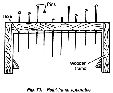
Fig. Point-frame apparatus
Requirements:
Point-frame apparatus, graph paper sheet, herbarium sheet, cello tape, note-book.
Point-frame apparatus:
A point-frame apparatus is a simple wooden frame of about 50 cm long and 50 cm high in which 10 movable pins are inserted at 45° angle. Each movable pin is about 50 cm long.
Method:
i. Put the point-frame apparatus (with 10 pins) at a place in the vegetation of grassland (Fig. ) and note down various plant species hit by one or more of 10 pins of the apparatus. Treat this as one sampling unit.
ii. Now put the apparatus at random at 10-25 or more places and note down each time the various plants species in a similar fashion. In case three plants of any species touch three pins in one sampling unit put at a place, the numerical strength of that particular species in this sampling unit will be three individuals. Write this value against the species below this sampling unit.
Observations and results:
Note down the details in the form of following Table 5:
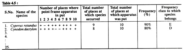
Now calculate the percentage frequency of each species as already done in Exercise No. 2. Allocate the various species among five frequency classes (A, B, C, D, E) mentioned in Exercise No. 4, find out the percentage value of each frequency class and prepare a frequency diagram as done in Exercise No. 4. Compare the thus-developed frequency diagram with normal frequency diagram.
Results:
Find out the three most frequently occurring species in the area studied. Also find out whether the vegetation is homogeneous or heterogeneous. Also try to determine the density values of individual species. Also find out at each place the total number of individuals of each species being hit by 10 pins of the point-frame apparatus.
8. Aim of the Experiment:
To prepare a list of plants occurring in a grassland and also to prepare chart along the line transect.
Requirements:
Two nails, 25 feet cord.
Method:
i. Prepare a 25 feet long line transect in a selected grassland by tying each end of a 25 feet cord to the upper knobs of two nails.
ii. Note down the names of the plant species whose projection touches one edge of the cord along the line transect, and assign all of them a definite number (e.g., 1,2,3,4, …etc.).
iii. Take