FINANCIAL ECONOMICS
(Modigliani, Markowitz, Merton Miller, Sharpe, Robert Merton and Scholes, Eugene Fama, Lars Peter Hansen, Robert J. Shiller)
Of the financial economists who received the Nobel Prize in Economics, Franco Modigliani was the first to receive the prize in 1985. He was followed by Markowitz, Merton Miller and Sharpe who received the Nobel Prize together in 1990. And in 1997, Robert Merton and Myron Scholes received the prize.
Franco Modigliani and Merton H. Miller are popular through their widely discussed theory named as Modigliani – Miller Theory (referred to here after as M and M theory). In their pioneering article “Dividend policy, Growth and The Valuation of Shares”, (in J.B. Oct, 1961) M & M have showed the irrelevance of dividend policy. M and M assumed a world without taxes, transaction costs or other market imperfections.
---------------------------------------------------------------------------------------
*Fn This Chapter is written by my daughter, Dr.V.Rama Devi, who has been working since June 2008 as Professor in the School of Management Studies, K.L.C.E.(KLCE became K.L. University in 2009, Guntur-2 (A.P.). Earlier, she worked as Associate Professor, College of Management, GITAM University, Visakhapatnam and as Asst. Professor at ICFAI University, Hyderabad. She is now working as Professor in Management in Sikkim Central University. An adapted version of this Chapter is published in Southern Economist, 1st Dec., 2008, Bangaluru.
The crux of MM’s position is that the effect of dividend payments on shareholders wealth is offset exactly by other means of financing. Where the firm has made its investment decision, it must decide whether to retain earnings or to pay dividends and sell the new stock in order to finance the investments. But the issue of an additional stock of shares will cause a decline in the terminal value of shares. What is gained by the investors as a result of payment of dividends will be neutralized completely by the reduction in the terminal value of shares. MM suggest that the sum of discounted value per share after financing and dividends paid is equal to the market value per share before the payment of dividends. In other words, the stock’s decline in market price because of external financing offsets exactly the payment of dividends. Therefore the investors according to MM will have no preference between getting the increase in wealth in the form of dividends now or capital appreciation later. The dividend pay out is irrelevant.
1) Irrelevance of Capital Structure:
Modigliani and Miller also showed the irrelevance of capital structure for investment decisions in perfect markets. The market value of a firm is independent of its capital structure. The sum of the parts must equal the whole; so regardless of financing mix, the total value of the firm stays the same, according to MM. The basic premise of MM approach is that, the total value of a firm must be constant irrespective of the degree of leverage
If the market values of any two firms differ then the process of arbitrage operates to equalize the values of the two companies. The central proposition of MM is that the weighted average cost of capital ( WACC) is independent of the debt-equity ratio and equal to the cost of capital which the firm would have with no gearing in its capital structure. MM argue that company value and the overall required return, Ko, are invariant to capital structure.
Markokwitz and Sharpe are widely known for their path breaking contributions to portfolio theory. According to Markowitz’s mean-variance maxim, an investor should seek a portfolio of securities that lies on the efficient frontier. A portfolio is not efficient if there is another portfolio with a higher expected value of return and with the same or a lower standard deviation or the same expected value with lesser risk. If inefficient portfolios are deleted, we get a set of efficient portfolios or efficient frontier. It is possible to draw a Risk-Return indifference map such that the investor is indifferent between any combination of risk and return on any indifference curve. The slope of the indifference curve is the investor’s marginal rate of substitution between risk and earnings. The point of tangency between the efficient frontier and the indifference curve is the optimal portfolio combination.
Markowitz devised an algorithm, using quadratic programming to calculate a set of efficient portfolios. His model is extremely demanding in its data needs and computational requirements.
Sharpe views that relationship between securities occurs mostly through their individual relationships with some index. This is known as Sharpe’s Index model. Sharpe’s model reduces the data requirement considerably.
In an article titled “A simplified model for portfolio analysis,” published in 1961, Sharpe relates each stocks return to the market as a whole rather than to every other stock. One way to capture this relationship is the market model. This can be expressed as
rs = ά + β rI + e
where rs = return on security
ά = intercept term
β = slope
rI = return on market Index and
e = error
This market model specifies that every risky security in a portfolio is related to the return on the market index such as SENSEX. The market model assumes that the return on a security is sensitive to the movements of the market Index (factor). Hence, the market model is also called Index model or Factor model.
Capital Asset Pricing Model (CAPM):
The CAPM shows the relation between risk and expected return for efficient portfolios. In the CAPM graph, we represent returns on the vertical axis and risk of the Portfolio on the horizontal axis. Efficient portfolios, plot along the line going from risk free return through the Market Portfolio. Efficient Portfolios consist of alternative combinations of risk and expected returns obtainable by combining market portfolio with risk free borrowing and lending. The lenear efficient set of the CAPM is known as the Capital Market Line (CML).
Because all investors face the same efficient set, the only reason they will choose different portfolios is that they have different preferences towards risk and return resulting in distinct indifference curves. Although the chosen portfolios will be different each investor will choose the same combination of risky securities. As a result each investor will spread his or her funds among risky securities in the same relative proportions, adding risk free borrowing or lending in order to achieve a personally preferred combination of risk and return. The tangency portfolio is referred to as market portfolio and it is same for all investors. Only there will be a certain amount of either risk free borrowing or lending that depends on that person’s indifference curves. The optimal combination of risky assets for an investor can be determined without any knowledge of the investor’s preferences toward risk and return. This feature of the CAPM is often referred to as the separation theorem.
In CAPM, the market will ultimately achieve equilibrium. In equilibrium the proportions of the tangency portfolio will correspond to the proportions of the market portfolio. The tangency portfolio is commonly referred to as market portfolio.
The vertical intercept of the Capital Market Line (CML) is the risk free rate of return which is often referred to as the reward for waiting. The slope of the CML is equal to the difference between the expected return of the market portfolio and the risk free security divided by the difference in their risk. The slope of the CML is often referred to as the reward per unit of risk borne. The intercept and slope of CML can be thought of as the price of time and the price of risk. In essence, security markets provide a place where time and risk can be traded, with the prices determined by supply and demand.
We have seen that the market model (Index model) uses market Index, whereas the CAPM involves the market portfolio. In practice the composition of the market portfolio is not precisely known; so a market Index must be used. As such beta determined by using market Index is used as an estimate of beta determined by market portfolio.
The Capital Market Line (CML) represents the equilibrium relationship between the expected return and standard deviation for efficient portfolios. The relation between covariance of security with the market and expected return is known as Security Market Line (SML). The securities with larger covariance with the market will be priced so as to have higher expected returns. Suppose the beta of an individual security is 1.5, the required rate on the market is 15% and risk free rate is 6% per annum. Then the required rate of return for the security is
0.06 + 1.5 (0.15 – 0.06) = 0.195 or 19.5%
The expected return for a security is the product of beta and the market risk premium plus the Risk free rate of return.
MYRON SCHOLES AND ROBERT MERTON:
In the 1970’s, Fischer Black, Myron Scholes and Robert Merton made a major contribution to the pricing of stock options. Before their work is recognised by the World, Black died. The remaining two received the Nobel Prize in 1997. Of their work, the most popular model is the Black-Scholes model. The Black-Scholes formula (BS formula) for pricing European Call Option on a non-dividend paying stock is given below. The buyer of Call Option gets the right but not the obligation to buy the Stock at a certain price. European call options can be exercised only on the expiration date only. The BSO formula for call options is given below.
C= S0.N(d1) – K. e–r.t . N(d2)
Where C is the value of the stock option
S0 is the current stock price at time zero.
K is the exercise price of the option
N (d) is the value of the cumulative Normal density function
e is an exponential, equal to 2.718
r is the short-term annual interest rate continuously compounded
t is the length of time to the expiration of the option, usually expressed as a proportion of an year
For the computation of d1 and d2, the formulas are
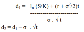
Where ln = The natural Logarithm
σ = The standard deviation of the annual rate of return on the stock
The BSO formula is taken from the well known text book by Hull. The formulas appear differently in other text books like Redhead book. But they are one and the same.
For Stocks providing a dividend yield at rate Q, the BSO formula for European Call options is modified on the basis of results derived by Merton. In the revised formula, Stock price is reduced from S0 to S0.e-QT where Q is dividend and d1 computation also changed accordingly.
The revised BSO (Merton) formula can be used for calculating European Call option for Stock Index. S0 is the value of the index and K is the exercise price of the index and Q is equal to the annualized dividend yield on the index.
For currency options also we use the same BSO (Merton) formula. We define S0 as the spot exchange rate and replace Q (dividend rate) with rf , foreign risk free interest rate.
In the case of American Call options on Stocks, the right to buy the stock can be exercised at any time upto the expiration date of the option. When there are no dividends on Stocks, the American and European Call option prices are equal and the BSO formula can also be applied to determine the price of American Call options on Stocks. When there are dividends on stocks, Black suggested an approximate procedure to determine the price of American Call option.
While the Call options give the right, but not the obligation to buy stock (underlying asset) at a specified strike price on a future expiry date, the Put options give the right but not the obligation to sell the stock at a specified price on a future date. So Put options are exact opposites of Call options. So BSO formula of Call options can be used for Put options also, by changing signs of formula C and rewriting the formula for Put option. The calculation of d1 and d2 remain the same.
The Global Financial crisis of 2008 has led to blaming the Financial models and question their underlying assumptions, that markets function efficiently. Actually, the financial industry consisting of Banks, Investment Funds, Hedge funds and such others are to be blamed for causing the Financial crisis. Fiscal stimulus policies and liquidity injection policies have averted the Financial crisis deepening into a Depression.
Eugene Fama, Lars Peter Hansen, Robert J. Shiller won the Nobel Price for 2013 for their work on predictions in Financial Market and also for spotting trends in Financial Markets.