Chandrasekaran, 1982). Two powerful methods for reducing the number of features are
approach described in section 5.2.
presented. These are the sequential forward search (SFS) algorithm and its backward
counterpart the sequential backward search (SBS) algorithm (Devijver & Kittler, 1982). The
5.2 Feature Selection Using the Sequential Backward Search Algorithm
pattern recognition system must also be capable of partitioning, or clustering, the reduced
The SBS is a top down approach, which starts with the complete feature set and removes
feature set into classes of similar observations. The K-means algorithm belongs to the
one feature at each successive iteration (Devijver & Kittler, 1982). The feature that is chosen
collection of multivariate methods used for classifying, or clustering, data and is presented
to be removed is the feature that results in the smallest reduction in the value of the
because of its general applicability in classification problems (Therrien, 1989).
selection criterion function when it is removed. In general, the SBS algorithm requires more
computation than the SFS algorithm because initially it considers the number of features in
5.1 Feature Selection Using the Sequential Forward Search Algorithm
the complete set as forming the subset. Although the SBS overcomes some of the difficulties
The SFS algorithm is a bottom-up strategy for removing redundant or irrelevant features
of the SFS approach the resulting feature subset is not guaranteed to be optimal.
from the feature matrix (Devijver & Kittler, 1982). At each successive iteration the feature
Furthermore, like its counterpart the SBS algorithm suffers from nesting because once a
that produces the largest value of the selection criterion function J is added to the current
feature is selected it cannot be disregarded. Implementation of the SBS approach is
analogous to the SFS approach detailed in section 5.1. The SBS algorithm is computationally
feature set. Given a set of candidate features Y R, a subset X R is selected without more expensive than the SFS algorithm, however, their performance is comparable. Despite
Texture Analysis Methods for Medical Image Characterisation
89
significant degradation to the classification system (Jain & Zongker, 1997). The best subset
X,
X x
i | i
,
1 2, , d,
xi Y,
(16)
of d features where( d ) D is selected from the set,
Y y j
D
1 |
1,2, , ,
(17)
by optimising the criterion function J, chosen here to be the estimated minimum probability
of error. For the set of measurements taken from Y, ideally the probability of correct
classification ( ) , with respect to any other combination, is given by,
i | i
,
1 2,,
d .
(18)
Fig. 10. Plot of fractal island area against cumulative number of islands acquired within the
It follows that the minimum probability of error for the space spanned by , for each class
area. The slope of the straight line plotted through the data is used to determine the fractal
i is defined as,
dimension.
(
E ) 1max( (
P |) ) (
p ) (
d
i
),
(19)
5. Feature Selection, Reduction and Classification
and the desired criterion function,
The texture analysis approaches presented in the preceding sections calculate features that
describe properties of the image, or region, being studied. This information is next used in a
J( X) min( (
E )).
(20)
pattern recognition system to classify the objects, or texture patterns of interest, into an
One of the disadvantages of the SFS approach is that it may suffer from nesting. That is,
appropriate number of categories or classes (Therrien, 1989). However, some of the features
because features selected and included in the feature subset cannot be removed, already
calculated may be highly correlated and some may contain irrelevant information. Feature
selected features determine the course of the remaining selection process. This has
selection is used to select a subset of features s from a given set of
s
noticeable hazards since after further iterations a feature may become superfluous. Another
p
p features such that p p
and there is no significant degradation in the performance of the classification system
limitation of the SFS approach is that in the case of two feature variables, which alone
(Therrien, 1989; Zongker & Jain, 1996; Stearns, 1976). The reduction of the feature set
provide little discrimination but together are very effective, the SFS approach may never
reduces the dimensionality of the classification problem and in some cases can increase the
detect this combination. To overcome this problem it is useful to start with a full set of
performance of the classification accuracy due to finite sample size effects (Jain &
available features and eliminate them one at a time. This is the method adopted by the SBS
Chandrasekaran, 1982). Two powerful methods for reducing the number of features are
approach described in section 5.2.
presented. These are the sequential forward search (SFS) algorithm and its backward
counterpart the sequential backward search (SBS) algorithm (Devijver & Kittler, 1982). The
5.2 Feature Selection Using the Sequential Backward Search Algorithm
pattern recognition system must also be capable of partitioning, or clustering, the reduced
The SBS is a top down approach, which starts with the complete feature set and removes
feature set into classes of similar observations. The K-means algorithm belongs to the
one feature at each successive iteration (Devijver & Kittler, 1982). The feature that is chosen
collection of multivariate methods used for classifying, or clustering, data and is presented
to be removed is the feature that results in the smallest reduction in the value of the
because of its general applicability in classification problems (Therrien, 1989).
selection criterion function when it is removed. In general, the SBS algorithm requires more
computation than the SFS algorithm because initially it considers the number of features in
5.1 Feature Selection Using the Sequential Forward Search Algorithm
the complete set as forming the subset. Although the SBS overcomes some of the difficulties
The SFS algorithm is a bottom-up strategy for removing redundant or irrelevant features
of the SFS approach the resulting feature subset is not guaranteed to be optimal.
from the feature matrix (Devijver & Kittler, 1982). At each successive iteration the feature
Furthermore, like its counterpart the SBS algorithm suffers from nesting because once a
that produces the largest value of the selection criterion function J is added to the current
feature is selected it cannot be disregarded. Implementation of the SBS approach is
analogous to the SFS approach detailed in section 5.1. The SBS algorithm is computationally
feature set. Given a set of candidate features Y R, a subset X R is selected without more expensive than the SFS algorithm, however, their performance is comparable. Despite
90
Biomedical Imaging
the shortcomings of the SFS and SBS techniques they are powerful techniques for reducing
The aim of the work presented in this case study was to develop a texture analysis
the feature set of real-world pattern recognition problems (Nouza, 1995).
methodology capable of distinguishing between the distinct pathology of the GTV and other
clinically relevant regions on CT image data. For eight bladder patients (six male and two
female), CT images were acquired at the radiotherapy planning stage and thereafter at
5.3 Classification Using the K-means Algorithm
The general clustering problem is one of identifying clusters, or classes, of similar points.
regular intervals during treatment. All CT scans were acquired on a General Electric single
For the specific problem presented in this chapter this would involve clustering the features
slice CT scanner (IGE HiSpeed Fx/I, GE Medical Systems, Milwaukee, WI, USA). Seven
calculated on a specific image region into a unique cluster. The number of classes may be
patients were scanned with a 3 mm slice thickness and one patient with a 5 mm slice
known or unknown depending on the particular problem. The K-means algorithm belongs
thickness. The repeat CT scans were registered against the corresponding planning reference
to the collection of multivariate methods used for clustering data (Therrien, 1989; Hartigan,
CT scan to allow comparison of the same region on each image. Image features based on: the
1975; Duda et al., 2001). The algorithm starts with a partition of the observations into
first-order histogram ( N 7) ; second-order GTSDM ( N 14) ; higher-order GLRLM
clusters. At each step the algorithm moves a case from one cluster to another if the move
( N 5) ; and a bespoke box-counting fractal approach ( N 1) were calculated on pre-
will increase the overall similarity within clusters. The algorithm ceases when the similarity
identified regions of the CT images of each patient (Nailon et al., 2008). Two classification
within clusters can no longer be increased.
environments were used to assess the performance of the approach in classifying the
bladder, rectum and a region of multiple pathology on the axial, coronal and sagittal CT
Assuming that the number of clusters N
image planes. These were, in the first using all of the available features ( N 27) and in the
c is known in advance the K-means technique may
be defined by the following three stages.
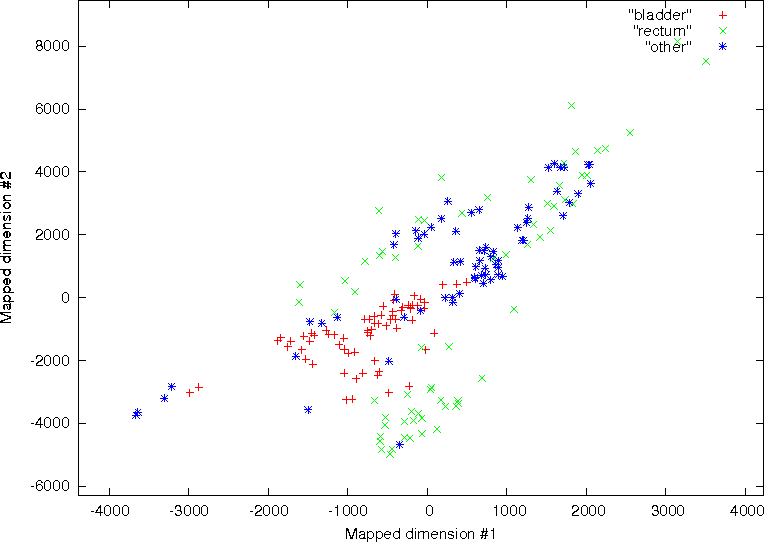
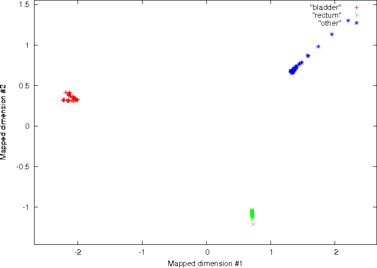
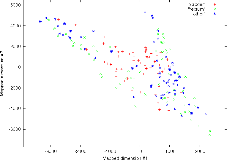
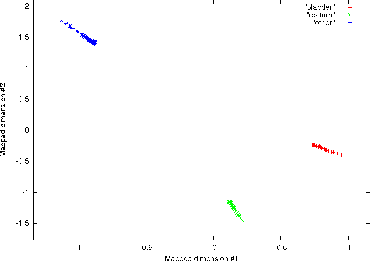
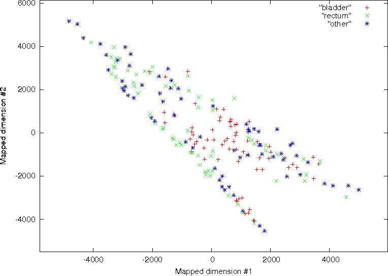
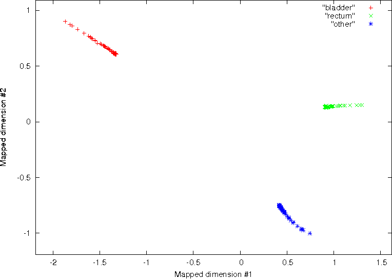
second using the best three features identified by the SFS approach. The classification results
Stage 1 – Initialisation: For the set of observations Y y , y , y to be classified into the achieved are presented in Fig. 11. No significant discrimination was observed between the
1
2
N
set of classes
, the algorithm starts with an arbitrary
bladder, rectum and the region of multiple pathology on the axial, coronal and sagittal CT
1 , 2 , , Nc
data using all of the available features ( N 27) . This is shown on the left column of Fig. 11.
partition of the observations into Nc clusters and computes the mean vector of
On the contrary, using the three best features identified by the SFS feature reduction
each cluster (
using the Euclidean distance
2
y where is the
approach, significant discrimination between the three pathological groups was possible.
1 ,
2 ,
Nc )
i
k
k
sample mean of the th
k cluster.
This is shown on the right column of Fig. 11. These results demonstrate the significant
Stage 2 - Nearest Mean: Assign each observation in Y to the cluster with the closest mean.
improvement in classification that can be achieved by removing features with little
Stage 3 - Update and Repeat: Update the mean vector for each cluster and repeat Stage 2
discriminatory power. Moreover the results demonstrate the effectiveness of texture
until the result produces no significant change in the cluster means.
analysis for classifying regions of interest, which may be difficult for the human observer to
interpret.
6. Biomedical Image Analysis Case Studies
The features that were found to work best were all from the GTSDM approach. The feature
produced by the bespoke box-counting fractal approach was not found to have significant
Two case studies are presented to demonstrate the practical application of the texture
discriminatory power. However, more research is required into the use of fractal methods in
analysis methods discussed in the previous sections. In the first, a texture analysis approach
this application area, particularly because assigning a single dimension to a whole region
was used to classify regions of distinct pathology on CT images acquired on eight bladder
may not be appropriate (Mandelbrot, 1977). Furthermore, the fractal dimension calculation
cancer patients. In the second, texture analysis was used to study the distribution of
may have been influenced by the different distribution of grey-levels in the images due to
abnormal prion protein found in the molecular layer of the cerebellum of cases of vCJD and
variations in the amount of urine in the bladder and air in the rectum.
sporadic CJD.
6.1 Case Study 1 - Texture Analysis of Radiotherapy Planning Target Volumes
The goal of radiotherapy, the treatment of cancer with ionising radiation, is to deliver as
high a dose of radiation as possible to diseased tissue whilst sparing healthy tissue. In
curative (radical) radiotherapy planning, delineation of the gross tumour volume (GTV) is
primarily based on visual assessment of CT images by a radiation oncologist (Meyer, 2007).
The accuracy therefore of the GTV is dependent upon the ability to visualise the tumour and
as a result significant inter- and intra-clinician variability has been reported in the
contouring of tumours of the prostate, lung, brain and oesophagus (Weltons et al., 2001;
Steenbakkers et al., 2005).
Texture Analysis Methods for Medical Image Characterisation
91
the shortcomings of the SFS and SBS techniques they are powerful techniques for reducing
The aim of the work presented in this case study was to develop a texture analysis
the feature set of real-world pattern recognition problems (Nouza, 1995).
methodology capable of distinguishing between the distinct pathology of the GTV and other
clinically relevant regions on CT image data. For eight bladder patients (six male and two
female), CT images were acquired at the radiotherapy planning stage and thereafter at
5.3 Classification Using the K-means Algorithm
The general clustering problem is one of identifying clusters, or classes, of similar points.
regular intervals during treatment. All CT scans were acquired on a General Electric single
For the specific problem presented in this chapter this would involve clustering the features
slice CT scanner (IGE HiSpeed Fx/I, GE Medical Systems, Milwaukee, WI, USA). Seven
calculated on a specific image region into a unique cluster. The number of classes may be
patients were scanned with a 3 mm slice thickness and one patient with a 5 mm slice
known or unknown depending on the particular problem. The K-means algorithm belongs
thickness. The repeat CT scans were registered against the corresponding planning reference
to the collection of multivariate methods used for clustering data (Therrien, 1989; Hartigan,
CT scan to allow comparison of the same region on each image. Image features based on: the
1975; Duda et al., 2001). The algorithm starts with a partition of the observations into
first-order histogram ( N 7) ; second-order GTSDM ( N 14) ; higher-order GLRLM
clusters. At each step the algorithm moves a case from one cluster to another if the move
( N 5) ; and a bespoke box-counting fractal approach ( N 1) were calculated on pre-
will increase the overall similarity within clusters. The algorithm ceases when the similarity
identified regions of the CT images of each patient (Nailon et al., 2008). Two classification
within clusters can no longer be increased.
environments were used to assess the performance of the approach in classifying the
bladder, rectum and a region of multiple pathology on the axial, coronal and sagittal CT
Assuming that the number of clusters N
image planes. These were, in the first using all of the available features ( N 27) and in the
c is known in advance the K-means technique may
be defined by the following three stages.
second using the best three features identified by the SFS approach. The classification results
Stage 1 – Initialisation: For the set of observations Y y , y , y to be classified into the achieved are presented in Fig. 11. No significant discrimination was observed between the
1
2
N
set of classes
, the algorithm starts with an arbitrary
bladder, rectum and the region of multiple pathology on the axial, coronal and sagittal CT
1 , 2 , , Nc
data using all of the available features ( N 27) . This is shown on the left column of Fig. 11.
partition of the observations into Nc clusters and computes the mean vector of
On the contrary, using the three best features identified by the SFS feature reduction
each cluster (
using the Euclidean distance
2
y where is the
approach, significant discrimination between the three pathological groups was possible.
1 ,
2 ,
Nc )
i
k
k
sample mean of the th
k cluster.
This is shown on the right column of Fig. 11. These results demonstrate the significant
Stage 2 - Nearest Mean: Assign each observation in Y to the cluster with the closest mean.
improvement in classification that can be achieved by removing features with little
Stage 3 - Update and Repeat: Update the mean vector for each cluster and repeat Stage 2
discriminatory power. Moreover the results demonstrate the effectiveness of texture
until the result produces no significant change in the cluster means.
analysis for classifying regions of interest, which may be difficult for the human observer to
interpret.
6. Biomedical Image Analysis Case Studies
The features that were found to work best were all from the GTSDM approach. The feature
produced by the bespoke box-counting fractal approach was not found to have significant
Two case studies are presented to demonstrate the practical application of the texture
discriminatory power. However, more research is required into the use of fractal methods in
analysis methods discussed in the previous sections. In the first, a texture analysis approach
this application area, particularly because assigning a single dimension to a whole region
was used to classify regions of distinct pathology on CT images acquired on eight bladder
may not be appropriate (Mandelbrot, 1977). Furthermore, the fractal dimension calculation
cancer patients. In the second, texture analysis was used to study the distribution of
may have been influenced by the different distribution of grey-levels in the images due to
abnormal prion protein found in the molecular layer of the cerebellum of cases of vCJD and
variations in the amount of urine in the bladder and air in the rectum.
sporadic CJD.
6.1 Case Study 1 - Texture Analysis of Radiotherapy Planning Target Volumes
The goal of radiotherapy, the treatment of cancer with ionising radiation, is to deliver as
high a dose of radiation as possible to diseased tissue whilst sparing healthy tissue. In
curative (radical) radiotherapy planning, delineation of the gross tumour volume (GTV) is
primarily based on visual assessment of CT images by a radiation oncologist (Meyer, 2007).
The accuracy therefore of the GTV is dependent upon the ability to visualise the tumour and
as a result significant inter- and intra-clinician variability has been reported in the
contouring of tumours of the prostate, lung, brain and oesophagus (Weltons et al., 2001;
Steenbakkers et al., 2005).
92
Biomedical Imaging
The approach was also found to be insensitive to CT resolution and slice thickness for the
data set studied. It was also noticed that discrimination of the bladder, rectum and other