Chapter 14—Analyze and abate project risks
In the pursuit cycle, the most urgent task of project risk analysis is to assist in determining the best bid amount. While in pursuit, you typically consider lower and lower bid amounts in the interests of achieving a competitive or better than competitive bid (see chapter 13). As the proposed bid amount gets lower, the probability of exceeding the planned cost and schedule will tend to increase. Moreover, the likely amount of the overrun also typically increases. At some point, the pursuit team will not want to further lower its bid amount due to fear of losing money and perhaps reputation and future credibility as well.
This situation pushes the pursuit team to reach a good understanding of just how bad the risks are for a given proposed bid. A prime question is how can the team know if the risks are excessive unless it somehow measures them? Gut feel is rarely a reliable guide!
Consider the insurance industry. Typically, an insurance company will not insure property against, say, fire damage, unless the property is in an area where there is considerable experience with the frequency and severity of fire. With a large experiential database, the insurance industry is confident that it can set rates for fire insurance that will allow it to pay all valid claims and still achieve a decent profit.
There is little about the kind of advanced projects dealt with in this book that an insurance company would even consider insuring, aside from its traditional areas of business. It would probably write “key person” insurance, fire insurance coverage for the buildings, and damage and liability insurance for the company cars and other properties. But it most likely would not touch writing insurance for the project’s maintaining schedule and staying in budget. With respect to those aspects of a project, the experience base simply is not there for doing the kind of actuarial analysis that insurance providers feel they must do in order to be assuredly profitable.
For similar reasons, contractors also might not want to take on these risks either. If the customer is willing to pay all costs, regardless of amount, contractors usually will be enticed to bid. That is why government agencies (especially for development contracts in the U.S.) and sometimes private companies sponsoring very risky but also crucial projects frequently offer a “cost plus fixed fee” (CPFF) contractual arrangement. In this arrangement the customer agrees to reimburse all costs, and the contractor pockets a usually smallish percentage fee that is tied not to the eventual cost outcome but to the bid amount.
When CPFF is offered, the contractor may be tempted to bid below what his costs will really be in order to improve his win probability. The contractor calculates that if the costs go higher, the customer simply will have to pay them. Too bad for the customer!
In past years, this has encouraged a considerable amount of under bidding, with bad results for customers. But in recent years, customers have gotten smarter. While they recognize that the risks may be too big for any contractor to bear, and CPFF is therefore appropriate, customers often cap their risks by telling the contractor the maximum funds available and refusing to go beyond that amount. Staying under the cap becomes the duty of the contractor, and if the contractor fails then he or she could wind up with a cancelled contract and an unhappy customer. This can reflect adversely on being awarded future contracts.
Also, customers have become more sophisticated at estimating true costs, thus narrowing the competitive range. Contractors must be similarly sophisticated so they can bid within it. As mentioned in chapter 8, analogy and parametric estimating have improved the ability of both contractors and customers to make realistic estimates in sophisticated projects.
Another way customers control their risks in CPFF situations is to reward the contractor for controlling costs. In this mode of contracting, contractors are awarded fees for good cost performance, and often for other good results as well, such as outstanding technical results, or for maintaining schedules.
If the customer and the contractor both feel confident that the contractor can succeed when given a fixed amount of money, the usual result is a fixed price contract. In this type of contract, if the contractor exceeds the planned costs, the contractor must absorb the loss. Often the contractor will also be penalized monetarily for not making the planned schedule.
Summarizing all this, it is important for bidders to understand their potential for loss at a given bid amount whether they are bidding in a cost plus or a fixed price environment, or somewhere in between.12 The potential for loss is more obvious in the fixed price situation, but losses can be real and damaging if the CPFF situation as well. For a given bid amount, the contractor needs to be able to estimate his confidence of adequate performance within that amount. The contractor also needs to know the potential losses that can arise. Having that information, the contractor must then decide whether or not the risks are acceptable.
Projects risks, like project cost estimates, can be approached by analogy or parametrically, or also using a bottom-up approach. In an analogy approach, what one typically does is to seek out completed projects of a similar nature and study the difference between what was bid and what the final outcome was. This can be tricky if there are numerous customer authorized changes in the course of the contract that allowed the costs to go up intentionally. The usual outcome of analyses of this sort is a range of percentage differences. For example, it might be found that cost overruns over the projects reviewed range from -10% to +40%.
If you are using a parametric model to estimate project costs, it often is the case that the model will have features that allow you to estimate a risk range at the same time. Again, you will wind up with a range of possible percentage overruns or under runs. By the way, if you use a parametric model, be sure you understand what risks it takes into account. Some parametric risk models do not account at all for some categories of risk. Also, depending on its architecture, it may or may not be of much help in management of risks.
The bottom up approach is much more labor intensive, but it also leads to a much better understanding of possible risk impacts. And it provides a basis for considering specific risk abatement approaches.
We recommend using the analogy or parametric approaches early in the pursuit cycle in the interests of speed of estimating. But before the proposal goes out the door, perhaps concurrently with doing a final bottom-up cost estimate, risk should be analyzed using the bottom-up approach, so that a credible risk abatement plan can be written. (Customers tend to love risk abatement plans when they have the ring of credibility. They don’t care much for them when they are full of clichés and generalities.)
Later in this chapter we will explore a particular approach to developing a bottom-up risk analysis and show how it can be applied to determining the suitability of a particular bid amount. But first we will explore doing that with a percentage range provided to us by either analogy or parametric methods.
Suitability of a given bid based on a percentage risk range.
The analysis presented here assumes a fixed price contract. The potential for loss is more clearly defined in fixed price than in CPFF contracts. But real losses are also possible in CPFF contracts, depending on circumstances.
Suppose you have used the Best Bid model (see chapter 13) to determine that to be competitive you need to bid $91.2 million on a particular project. You have three competitors (N = 3) and according to the model, a bid of $91.2 million will provide a competitive win probability of 0.25 (25%) given the competitive pressure in the bidding environment.
You have estimated the costs (without contingency or profit) of your current baseline project (product plus programmatic) design at $75 million. You have determined the competitive bidding range to be $85 t0 $115 million.
The $75 million cost estimate is just that, an estimate. Based on analogies with completed similar projects, you determine that the actual cost could be anywhere between $70 million and $100 million. This corresponds to an estimating error ranging from -6.7% to +33.3%. (Estimating error ranges of this magnitude should never be realized in routine contracting, such as most construction, but surprisingly they often are! In high tech or other non-routine contracting they are not at all uncommon.)
The next stage of your analysis assumes that all outcomes between $70 and $100 million are equally likely. This may not be true, but if you lack evidence to the contrary the Principle of Insufficient Reason (explained in chapter 13) makes it the most reasonable assumption.13 The situation is shown in Exhibit 14-1.
In the exhibit you see your current cost estimate of $75 million, the competitive range of $85-100 million, and the competitive bid of $91.5 million, yielding a win probability of 25%. Also in the exhibit is the range of cost uncertainty, $70-100 million, and a plot of win probability versus bid amount developed from the Best Bid model.
Exhibit 14-1—Hypothetical Bidding Risk Analysis
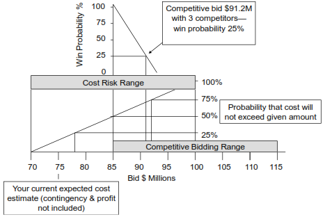
The diagonal line rising across the range of cost uncertainty represents the probability that the cost will not exceed the amount obtained by dropping a vertical line down to the bid axis. (Technically, it is a cumulative distribution function.) For example, the probability that the cost will not exceed $78M is 25%; the probability that the cost will not exceed $85M is 50%, and the probability that the cost will not exceed $92M is 75%. (Depending on how it is derived, this line will not always be straight. An S-shaped line is likely if a distribution other than uniform is used.)
If you bid $91.2M you are competitive, but what is your picture with respect to risk? At a bid of $91.2M, the plot says that the probability of the cost not exceeding that amount is about 74%. Looking at it from the opposite point of view, it says you have about a 26% chance of losing some amount of money because costs exceed $91.2M.
Suppose that your company is averse to losing any money on fixed price contracts, and will accept no more than a 10% probability of this happening. You would go to the 90% point on the diagonal line and find that you would have to bid on the order of $97M (reading the curve approximately). Unfortunately, this would reduce your predicted win probability to almost zero. You would have three options:
Let’s look at another hypothetical situation. Suppose your company hires a new general manager a month before the bids are to be submitted and she is less risk averse than the old one. In her view, a 20% chance of overrun loss is acceptable on this project because the project will give you access to new technology that you would not otherwise have. The future benefits of this technology she perceives to be huge.
The exhibit shows that a 20% chance of loss corresponds to a bid of about $94M, and a win probability of around 10%. On being informed of this, the new general manager decides that she is willing to accept even larger potential losses to gain the new technology. She wants a 50% win probability. With the current cost and risk structure, this corresponds to a bid of about $88M. But she also wisely orders that more studies be done to try to further reduce both costs and cost uncertainty. In addition, as a precaution, she orders that the reasonableness of the low cost approach finally adopted must be carefully explained to the customer against the possibility that the customer could perceive it as an attempt to “buy in.”
The above analyses are perhaps a bit overly simplified from what a real analysis would be like, but are indicative of the general approach.
A point to remember: Costs and cost risk are real and must be considered in bidding, but profits and contingency amounts to be included in bids are optional! In truth, the amount of profit realized from a project depends not on how much “profit” we include in the bid, but on how well we control project costs and risks. Moreover, sometimes we are willing to forego immediate profits for the sake of long term objectives, among them survival and improved competitive position in the future.
Risk drivers and bottom-up risk analysis
Simple assumptions suffice for bid analysis early in the pursuit cycle. But as the time nears to present the proposal, a more detailed bottom-up risk analysis should be performed for several reasons. Here are three:
Many systems have been advocated for doing project risk analysis. The scope of this book does not allow for inclusion of descriptions of them. Here we will limit the discussion to one approach that will result in a probability distribution that can be used in an analysis similar to that portrayed in Exhibit 14-1. The approach shown is limited to cost risk because that is most germane to the bidding problem. Other types of risk that are often considered in risk analysis are schedule risk and risks of failure to accomplish technical objectives.
The method requires that a work breakdown structure (WBS) be defined for the project (this was discussed in Chapter 9, but see also Appendix D). Only the ultimate children (“leaves” or “tips”) of the WBS tree are considered.14 They should be formed into a list with their cost estimates stated and summed. The cost estimates should be the honest most probable costs, as judged by the team. They should be neither “fat” nor “lean.” Obvious contingencies should not be included.
The next step is to identify “risk drivers.” For purposes of this book, the following definition applies:
A risk driver is a root cause force or circumstance that may act to change the cost of one or more tasks in the project.
That it be a root cause rather than merely a symptom or a proximate cause is important.15 Using symptoms or proximate causes as proxies for risk drivers causes logical and statistical entanglements that can invalidate the analysis. This is because a symptom may result from several risk drivers acting concurrently. Also, a risk driver may produce more than one symptom. Risk drivers are typically identified using bottom-up processes such as brainstorming and various checklists, followed by cause and effect analysis.
We must have a project plan before we can assess risk, but do we need a “complete” plan? Can we make do with a sketchy plan? The level of detail in a plan that is most appropriate for assessing risk is generally less than the detail needed to assure that everybody knows what to do at a particular time. Plans for major projects seldom have a temporal resolution of less than one week, unless an important activity inherently requires less than one week. But for analysis and management of risk, we generally want to use a condensed plan that omits a lot of detail. Such a plan generally will have 100 or preferably fewer “activities.” It is the kind of high-level summary plan that is typically presented in management briefings. Bottom up risk analysis in a project plan showing many hundreds or even thousands of detailed tasks is impossibly tedious.
Each risk driver must be assigned a probability of occurrence. This is a number in the range 0-1 or equivalently a percentage range 0-100%. This number is assigned subjectively by the project team or by selected members of the team. The same group that assigns the probabilities also assigns a cost impact range to each project task due to each risk driver, given that it happens. This information is then combined with the list of tasks to form a matrix such as shown in Exhibit 14-2:
Exhibit 14-2—Example Risk Analysis
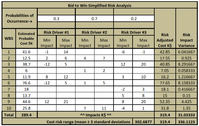
In this exhibit, the risk drivers are represented by “min” and “max” impact values with respect to each task, and also by probability of occurrence values. The impacts are assumed to occur only if the risk drivers occur. The combined effects of each risk driver are collected in the columns headed Risk Adjusted Cost $K and Risk Driver Impact Variance. (For readers with a background in statistics, the risk adjusted cost is a “mean” or “expected value,” and the variance is the square of the standard deviation. For simplicity, each risk driver range is assumed to represent a uniform distribution of the cost impacts.)
The $289.4K figure represents the total cost the team would have used in its plan in the absence of risk. The total $319.4K represents a risk adjusted “expected” cost. The difference of $30K is the likely overrun if risk is not considered in setting the bid amount.
Two other numbers are produced by the mathematics underlying the table. They are the cost risk range, namely $302.7K to $336.1K. These are produced respectively by subtracting three standard deviations from the risk adjusted amount and adding three standard deviations to it. Readers who have taken “Business Statistics 101” will recall that typically the mean plus and minus three standard deviations includes most possible outcomes. There is only a very small probability of being outside this range.16
An S-shaped cumulative probability curve for Exhibit 14-1 could be drawn by assuming that the results from Exhibit 13-2 are normally (or better, lognormally) distributed. See any decent college level business statistics text for further details.
Risk abatement in bidding
In a pursuit we potentially can talk about three kinds of risk abatement:
These three kinds of risk abatement form the basis of your project risk management plan. If required by the customer, this is submitted with the proposal. If not required by the customer you should prepare it anyway for your own use. (Sometimes a customer will be fascinated that you have one and will be pleased to see it even if the customer did not require it.)
A recurring issue raised by pursuit managers is the fear that if you submit a realistic risk management plan and the competition plays down the risks, you will frighten the customer and lose out in the bidding. This is sometimes a realistic fear. The answer is to know your customer (chapter 2). If there are real risks in the project that are common to all competitors, and your customer has failed to see them, they should be discussed with your customer long before the request for proposal is issued. The customer will then not be surprised to see them discussed in the proposal. In fact, the customer will be surprised if they are not discussed.
If the risks are peculiar to your project design, they could be ignored or understated in the proposal, but the risk in that is that one or more competitors may spot your vulnerability and use it to flog you in their proposal. This might be more damaging than a forthright statement of the risks and your means for dealing with them.
Customers today are often quite astute about risks and their potential impacts on the project. If your customer is astute in this area, one thing worse than honestly admitting to serious risks in your proposal is to attempt to cover them up. Worse still is not to be aware of them.
We always advocate that the project team statistically quantify its risks on all large or complex projects, but this does not necessarily mean that a quantified risk analysis should be presented to the customer in the proposal. For many customers this is overkill. For customers ill equipped to deal with statistical analyses, we recommend a simple “high, medium, low” approach to risk description. But we do always recommend the identification and description of root cause risk drivers for customers, and at least a general, non-quantitative discussion of their possible effects.
Most efforts at risk abatement boil down to one or a combination of the following ten activities:
Allocation of risks among stakeholders
We conclude this chapter on analyzing and abating project risks with a question any project stakeholder should ask: Whose risk is it? Projects can be structured in any number of ways. Many types of relationships can exist between stakeholders. Some risk drivers may damage or benefit some stakeholders more than others.
The ideal arrangement in any project is when risk is allocated to the stakeholder best able to manage it.
“Managing” it includes having the resources to pay for bad outcomes that happen in spite of everyone’s best efforts. Poor allocation of risk is itself potentially a risk driver, because if a bad thing happens to a project team member (e.g., a subcontractor) who is vulnerable, the subcontractor may fail, and bring the project down.
There are many devices for distributing risk. A success-oriented project should look for a win-win selection of these devices. Here are a few: