Bid to Win: A Guide to Pursuit, Capture, and Management of Unprecedented or High Technology Projects by Evin Stump - HTML preview

Appendix C -- Miscellaneous tools

Here we present several tools that can be helpful in bidding to win. These are tools of wide application. As they are described, we will point out possible uses.

• Brainstorming. A tool for developing information based on “hidden knowledge” and intuition.
• Multivoting. Brainstorming frequently generates a long list of possibilities.
• Multivoting provides a means for prioritizing them.
• Ishikawa diagrams. Ishikawa diagram were invented by Kaouru Ishikawa. They are also known as fishbone diagrams or cause-and-effect diagrams. They are useful in determining underlying or root cause of risks and problems.
• Pareto principle. This is also known as the 80-20 rule, or the law of the vital few. It is widely used in many areas of life and work.
• Analytic Hierarchy Process. Invented by Dr. Thomas L. Saaty at the University of Pittsburgh, this is a powerful tool for quantifying the relative importance of a number of alternatives as ratios.
• Variation analysis. This a mathematical method for dealing with a frequently arising problem: what is the cost of accuracy? What premium do we have to pay to increase accuracy? What can we save by loosening up quantitative tolerance requirements on products? We speak here not just of dimensional tolerances but accuracy requirements of any type.

Brainstorming

Brainstorming is a group method for generating ideas, which can be inputs to other methods for screening, grouping, prioritizing, or evaluating. It is particularly valuable for identifying risk or cost drivers, design alternatives and other information which lies hidden beneath our conscious thoughts.

Here are some characteristics of brainstorming:

• Often used for identification, but can also be useful for analysis, tracking, controlling, etc.
• Participants verbally identify ideas; participants may build on each other’s ideas (“chaining”)
• Best used in a small group (<10 people)
• Requires a tactful facilitator to deal with conflict and to encourage shy people to participate
• Does not require participant training
• Is an enjoyable exercise
• Generates a lot of ideas in a short time

Here are suggestions on conducting a brainstorming exercise:

• Facilitator explains subject matter, process, and the rules:
• Do not judge or criticize ideas of the speaker.
• Encourage wild ideas and out of the box thinking.
• Build on ideas of others (“chaining”).
• Go for quantity of ideas; don’t try to develop ideas into plans or root causes (do that later).
• Participants generate ideas using one of two processes:
• Unstructured: call out ideas spontaneously.
• Round-robin: each participant takes a turn, in order, to state an idea (forces shy people to contribute).
• Record ideas—facilitator writes on a visual medium in sight of all participants
• Review list—all review for clarity and understanding; revise as needed.

As an alternative to “free-form” brainstorming, it is sometimes helpful to do a more structured version. In structured brainstorming, the group starts with a short memory-jogging checklist. They begin at the top of the list, and generate ideas about each item in the list, in turn, until no more ideas seem to be forthcoming. At that point, the facilitator moves on to the next item on the list.

Multivoting

The output of a brainstorming session more often than not is a rather long list of possibilities. Generally, the list will be too long to consider all of them in detail. It is necessary to screen the list and determine which items in it are possible winners and which are likely to be losers. Multivoting is a method for prioritizing and shortening a long list.

In the literature you can find more than one definition of multivoting. The description given here is a popular one, but not the only one. If you are interested in looking at other versions, you can find them on the Internet.

Here are the steps for the version we prefer:

• Using brainstorming (or some other method), form a list of possibilities. The order they are in is not important at this stage.
• Create a multivoting caucus, a group of people that has high interest in and familiarity with the subject matter. A practical limit to the number of people in the group is about ten. Three is a good minimum. A disinterested facilitator should lead the group.
• Have the items displayed visibly, perhaps on a chalk board. Sequentially number all of the items in the list of possibilities beginning at 1.
• The facilitator should go over every item in the list with the group to make sure everyone has the same understanding of it.
• Determine the number of items each person in the group will be allowed to vote for. A good choice is approximately one-third of the number of items in the list. For example, if the list contains 23 items, seven would be a good choice. Whatever that number is, let’s henceforth call it N for convenience.
• Have each person in the group vote for the N items in the list he or she considers “best.” The most convenient way to do this is to have each person write down on a piece of paper the N numbers that identify their choices. The facilitator shall collect these initial votes.
• The facilitator shall put a checkmark in front of each item for each vote it receives.
• Reduce the length of the list to a length desired by the group. A convenient way to do this is to first cross out all items that got no votes. If that isn’t short enough, cross out all items that got just one vote, and so forth.
• If agreeable with the group, the remaining items can be prioritized by how many votes they got. Ties can be broken by a show of hands. If any issues remain, the multivoting can be repeated, perhaps with the number of votes per person reduced.

Ishikawa diagram

An Ishikawa diagram, also known as a fishbone diagram, or as a cause and effect diagram, is a useful tool for finding root causes. When do we usually want to do this? Two situations: 1) problems, and 2) risks.

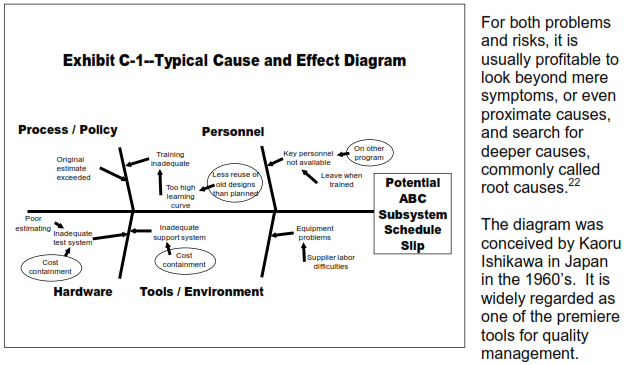
Obviously, the name fishbone diagram comes from its resemblance to the pattern of bones of a fish. The architecture of a fishbone diagram is as follows:

• On the right, a box is drawn. Into this box is put a brief statement of the problem or risk of concern. The example above concerns a risk. A risk can be distinguished for a problem by the presence of a conditional word, such as “may,” “might,” “could,” “possible,” or “potential.”
• A main bone is drawn on the left, terminating at the box.
• Two or more rib bones are drawn diagonally, leading into the main bone. Above we have drawn four. Each of these is labeled with the name of an area from which proximate causes are believed to originate. There is considerable flexibility in naming these. Above, the ribs are labeled
• Process/Policy
• Hardware
• Personnel
• Tools/Environment
• By some method, usually brainstorming, first assign the most obvious proximate cause. Add branches off the proximate causes until an agreeable root cause is identified – agreeable in the sense that something might be done to fix it and thereby mitigate the risk.

Pareto Principle

The Pareto principle, named after the Italian economist Vilfredo Pareto, is also known as the 80/20 rule. It states that in many situations, 80% of the outcomes stem from 20% of the causes. For example, it is frequently held to be true that 80% of a product’s cost is determined by the first 20% of the design decisions.

What led Pareto to announce his principle was his observation that 80% of the wealth of Italy was held by 20% of the population.

The rule is a useful approximation to reality for many situations, and can be an aid to analysis. However, it is not true for every situation and one must be careful not to misuse it.

Analytic Hierarchy Process (AHP)

AHP, an invention of Dr. Thomas L. Saaty of the University of Pittsburgh, is a process widely used in planning, priority setting, and resource allocation. A virtue of the process is that it can reduce very complex decision making situations to a relatively simple pair-wise comparison of options.

Our description of it here will not even touch on the full range of its capability. We will describe its use in fairly simple situations. Readers interested in learning more about it are referred to the text “The Analytic Hierarchy Process,” by Thomas L. Saaty (RWS Publications, Pittsburgh, PA).

AHP is a mathematically reasonable and robust way to handle human judgments in complex decision situations. For example, suppose we are not able to get direct and decisive information about a customer’s relative preferences for various project goals. But we are able to get testimony from various people who have been in close contact with the customer. One simple thing they could do is to agree on how the customer would rank the goals in an ordinal sense, which is just a fancy way of saying that they can make a list of the goals in order of the customer’s preference. That of course is valuable knowledge, but even better would be to know the customer’s preferences in the ratio or quantitative sense.

Suppose for example, that the product is an aircraft and the major goals are only three in number: airspeed, altitude and payload. Further suppose that the ordinal ranking is:

• Payload.
• Airspeed.
• Altitude.

But we want to know more. Is payload twice as important as airspeed? Is airspeed only marginally preferable to altitude? AHP helps us find these answers.

The technique is based on making pair-wise comparisons and forming them into a specific kind on matrix called a reciprocal matrix. That part is easily explained and we will do so shortly. It’s the part beyond that which is harder to explain because it involves some mathematics that most people never encounter, even some engineers and scientists. But for the mathematically sophisticated among our readers, the process involves finding the dominant eigenvalue of the matrix and also its corresponding eigenvector. Fortunately, you don’t need to be able to actually do this sophisticated math to use AHP. If your problem involves finding the ratio ranking of only three, four, or as many as five parameters, you can use an AHP spreadsheet program that is included in our CD that can be ordered by readers of this book (see the final page of the book). If you are even a bit sophisticated with spreadsheets you can easily expand the method on this spreadsheet to six, seven, eight or more parameters you want to rank. Beyond about ten parameters, AHP becomes difficult because of the mental challenge of keeping all of the comparisons straight.

Now that we have ducked the hard part of the problem by referring you to software, we can comfortably and rather painlessly talk about the process of forming the requisite reciprocal matrix. Suppose we have four parameters to rank, call them A, B, C, and D. We form a 4x4 matrix like this (Exhibit C-2) with 1’s in the main diagonal:

Exhibit C-2—AHP Matrix Example (Initial Condition)

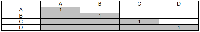
Then we proceed to make all possible pair-wise comparisons, preferably in a random fashion.

Suppose our first comparison is between A and C. If we (an individual or a group) believe that (say) A is more important than C, we have to decide approximately how much better. We express that preference on a scale of 1 to 9, defined as follows.

• If A and C are equally important, enter 1 into the cell that is the intersection of the A row and the C column. (Note that this is the reason all the cells in the main diagonal have entries of 1. For example, A is as important as itself.)
• If A is weakly more important than C then insert 3.
• If A is strongly more important than C then insert 5.
• If A is very strongly more important than C then insert 7.
• If A is absolutely more important than C then insert 9.
• If you have trouble deciding which of the above odd numbers to insert, then insert the intermediate even number. As an example, if you are undecided between 3 and 5, then insert 4.

The above explains what you do if the row parameter is more important than the column parameter. If the reverse is true, for example if C (row) is less important than D (column). then insert the reciprocal of 3, 5, etc.

You only need to fill in the empty white cells in Exhibit C-3. The main diagonal cells already are filled with 1’s. To fill the remaining cells, the spreadsheet software will automatically insert the reciprocals of the corresponding cells across the diagonal.

Exhibit C-3 is an example of what a filled in matrix might look like.

Exhibit C-3—Example AHP Matrix (Filled In)

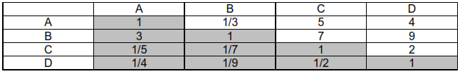
Obviously, in filling in such a matrix, one must be careful to be as consistent as possible For example, if one were to say that A is more important than B, and B is more important than C, then it wouldn’t do to say that C is more important than A.

It’s hard to be perfectly consistent, and it gets even harder as the size of the matrix increases. Fortunately the AHP mathematics provides you a method for determining whether or not inconsistencies are in reasonable bounds. It calculates a value called the consistency ratio (CR). If CR<0.1 then consistency is acceptable, according to Dr. Saaty. If the consistency ratio is too high, it’s generally easy to go back to the matrix and find the problem then correct it. Some commercially available AHP software (but not our free spreadsheet!) helps you find inconsistencies.

Plugging the matrix above into the spreadsheet yields CR = 0.04 (consistent enough) and the following quantitative rankings:

A = 4.76

B = 10.75

C = 1.44

D = 1

Thus, A is 4.76 times as important as D, B is 10.75 times as important, and C is 1.44 times as important. Likewise, A is 4.67/1.44 = 4.24 times as important as C.

This method is powerful and widely accepted. We recommend it for any situation where it is necessary to rank a small number of parameters quantitatively based on human judgment.

Variation analysis

We must give warning. This is the most mathematically sophisticated section of this book. You may not want to tackle it unless you have a background in mathematics up to and including calculus and statistics. We assume that this subject is of most interest to engineers and scientists and that they will have the mathematical skills to understand the development.

This is a book about bidding to win. Much of the discussion is about product cost and keeping it low. There is also emphasis on minimal design, that is, design that just meets customer goals without adding gold plating. The present discussion further promotes that emphasis.

To introduce the method called variation analysis, we present a simple example. Once you understand this example, you may find the method useful in more complex problems. It has been used by several project teams in problems far more complex than the simple example shown here.

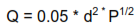
Consider a situation where an orifice will be used to closely control the amount of flow of a liquid in a machine. Hundreds of the machines will be built and sold. We want the cost to be as low as possible. The rate of flow through the orifice Q is governed by the following equation which has been derived from accepted principles of fluid mechanics:

Q = 0.05 d2 P1/2

Here Q is the rate of flow in cubic feet per second (cfs), d is the diameter of the (round) orifice in inches and P is the upstream pressure in pounds per square inch (psi). Note that only d and P control Q. If Q must be controlled accurately, then the accuracy of Q will in some sense depend on the accuracy of d and P.

Shortly we will explore how this can be evaluated. But first we take note of a well known phenomenon in industry—accuracy costs money. Following the principle of minimal design enunciated in chapter 10, we don’t want any more accuracy than we need to satisfy customer goals. This notion goes against the grain with many design engineers, who are culturally prone to putting expensive accuracy requirements into drawings and specifications, apparently out of habit. Some even think this is good engineering.

If the accuracy of more than one parameter must be considered in determining the accuracy of the product (as is the case with the orifice discharge problem we are considering), then a tradeoff may exist as to which parameters can most beneficially have looser tolerances in order to keep costs down. Such will turn out to be the case with our simple orifice example.

The relationship between cost and accuracy can take several forms, anywhere from a simple straight line relationship to a curve with a knee as illustrated in Exhibit C-4.

Exhibit C-4—Typical Curve with Knee

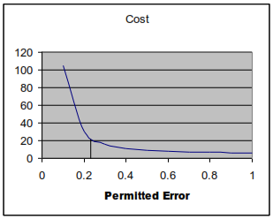
(Note: the numbers on the axes in Exhibit C-4 have no significance. They are for illustration only.) When the cost vs. permitted error relationship has a pronounced knee as in Exhibit C-4, it’s important to try to stay to the right of the knee if at all possible. In this example, note that if we allow permitted error to be greater than about 0.23 (note the short vertical line in the exhibit), costs remain below 20 (arbitrary cost units). And they change only gradually as tolerance of error changes. There’s not much difference in cost between a permitted error of 0.5 and 0.6. But if permitted error is forced to go below 0.23, costs rise sharply. There is a huge difference in cost between a permitted error of 0.2 and 0.1. This is illustrative of the knee of the curve phenomenon that occurs in many tradeoffs of cost versus accuracy.

Let us suppose that the nominal pressure we will work with is 10 pounds per square inch and that the nominal diameter of the orifice is 2 inches. The pressure will be controlled by a purchased pressure regulator and the orifice will be shaped by internal grinding of a hole in a steel plate. Based on the above formula the flow we will achieve with this diameter and this pressure will be:

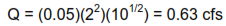
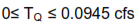
Let us further suppose that we need to keep the flow within 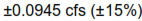of this value in order to meet customer goals. This requirement clearly will drive the tolerances we must impose on d and on P, and will also drive the cost we must pay because accuracy is expensive. But we will want to keep the cost as low as possible.

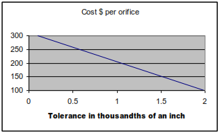
Suppose we find that tolerances as tight as inches for the orifice are readily obtained for $100 an orifice (this is hypothetical, of course).23 We assume that looser tolerances do not significantly decrease cost. But for tolerances tighter than inches costs increase significantly. We find after a bit of research that the following linear equation closely approximates the cost effect for tighter tolerances.

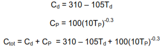
Orifice cost $ = 310 – 105*(tolerance in thousandths of an inch)

The tightest practical tolerance is inches, so our range of interest is from inches to inches. Cost per orifice over this range of interest is plotted in Exhibit C-5.

Exhibit C-5—Cost of Orifice vs. Tolerance

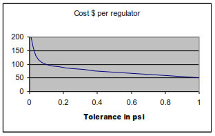
We next consider pressure regulators. Let us (hypothetically) suppose that a survey of vendors turns up suitable regulators with accuracy of regulation ranging from 0.1% to 10% of the desired pressure. After obtaining several vendor quotes and doing a regression analysis on the resulting data we determine that the following equation is a good fit to the data:

Regulator cost $ = 100*(10*regulation error in psi)-0.3

Exhibit C-6 plots the regulator cost versus the error in psi.

Exhibit C-5—Cost of Regulator vs. Tolerance

Now we introduce the means for connecting the errors in the orifice and in the pressure regulator to the errors in the flow quantity. It is known to statisticians as the propagation of error formula. Although it probably is of most interest to engineers and scientists, it is not discussed in many statistics texts written specifically for engineers and scientists. Readers interested in further pursuing it may have to look in several books to find it. Our source is “Basic Statistical Methods for Engineers and Scientists” by Neville and Kennedy, second printing, published in 1966 by International Textbook Company, Scranton, PA.

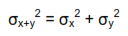
Readers having some familiarity with statistical methods may recall that if two random variables are independent, then the variance of their sum is equal to the sum of their variances, thus:

This is a special case of the more general propagation of error formula that is not limited to sums. It can cope with many types of continuous functional relationships and can deal with two or more variables that contribute to error. The expression of this relationship we will use is:

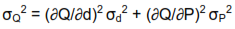
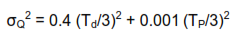
The propagation of error formula as applied to our flow control example states that the variance in flow is equal to the variance in orifice diameter multiplied by the square of the partial derivative of Q with respect to plus the variance of P multiplied by the square of the partial derivative of Q with respect to P.

As previously noted, we have a formula relating Q to d and P, namely:

Taking partial derivatives, evaluating at the nominal diameter and pressure and squaring the results leads to:

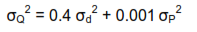
Note the coefficients of the variance terms on the right hand side of this equation. The coefficient 0.4 is 4,000 times the size of the coefficient 0.001. This is a clue that the error in diameter of the orifice will be of much more significance than the error in regulated pressure. Mostly this is due to the fact that diameter is squared in the underlying equation, while the influence of pressure varies only as the square root. In general, the error effects of variables that are raised to higher powers or that are exponential in nature will have more impact than linear variables or variables that are raised to lower powers. This intuitively makes sense.

How do we evaluate the variances on the right hand side of the formula? We can consider both d and P to be normally distributed with means 2 inches and 10 psi respectively, and consider their variances to be related to the tolerances we impose. For example, suppose we impose a tolerance of inches on the orifice diameter. Because of the assumption of a normal distribution, we can conveniently consider 0.001 inches to be equivalent to three standard deviations (see any decent introductory text on statistics). One standard deviation is therefore 0.001/3 = 0.00033 in. The variance is defined as the square of the standard deviation, therefore assigning a tolerance of in results in a variance of (0.00033)2 or 1.111E-7 in2.

We can easily construct a simple formula for what we just demonstrated.

Here T is the one-sided tolerance we have imposed. By one-sided we mean that if we have imposed inches, then T = 0.001. This formula is perfectly general and is valid for the assumption of a normally distributed error. It is reasonably accurate for many non-normal distributions that occur in practice.

We can now rewrite our previous equation in terms of assigned tolerances:

We are ultimately interested not in the variance of Q, but in its standard deviation. We can obtain that by taking the square root of the above. At the same time, we convert to its tolerance equivalent using

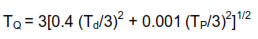
Let’s define two additional variables:

Cd = cost of one orifice of diameter d

CP = cost of one pressure regulator

We can now write two previously developed equations in terms of our newly defined variables, and create yet another useful equation, this time for the total cost, Ctot:

Let’s summarize what we have done to this point. We have developed the following two equations that we will use to minimize total cost:

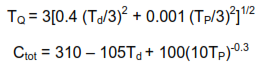
We have also established the following constraint:

Additionally we have established the following practical ranges that are effectively constraints:

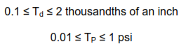
What we now have is a rather complicated constrained nonlinear optimization problem in which we want to minimize Ctot subject to constraints on TQ, Td, and TP. Elegant techniques exist for solving such problems, and in a more complex problem than this one their use may be warranted. Here we will use a very inelegant approach. We will create a spreadsheet containing both the TQ equation and the Ctot equation and proceed by trial and error by entering various values of Td and TP within their allowable ranges. There is no guarantee that this method will find an absolute minimum but it can come very close with a few minutes of exploration of the trade space.

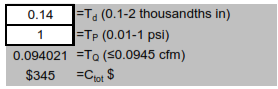
In the particular problem we are dealing with, the cost is much more sensitive to orifice diameter than to pressure control. Our intuitive trial and error search strategy begins by using the cheapest regulator then tightening the diameter tolerance until the constraint on Q is met. Then we explore that vicinity until the constraint is satisfied and we get the lowest cost we can find. Exhibit C-7 shows the simple spreadsheet we used in this search, and the solution we quickly found.

A second approach was to use Monte Carlo simulation in a spreadsheet to rapidly try many combinations of tolerances. This approach is essentially computer-aided trial and error. The best solution we found in 5,000 simulations was less than a dollar away from  our intuitive solution, but when a problem gets more complicated than this simple example Monte Carlo will be far more reliable and faster than an intuitive search.

The simulations ran in less than a minute. We did have to spend about an hour programming a macro in the VBA language to automate the Monte Carlo.

Exhibit C-7—Manual Search Spreadsheet

Minimization of total cost

In closing, we should note that engineers generally do a good job of developing the basic design solution. Where they are most likely to go wrong is in developing a solution that is too good. This can raise costs and damage chances of having the winning bid. The method of variation analysis can make a unique contribution to avoiding that unfortunate situation.