Chapter 3
Floating-Point Numbers
3.1 Introduction1
3.1.1 Floating-Point Numbers
Often when we want to make a point that nothing is sacred, we say, one plus one does not equal two. This is designed to shock us and attack our fundamental assumptions about the nature of the universe. Well, in this chapter on oating- point numbers, we will learn that 0.1 + 0.1 does not always equal 0.2 when we use oating-point numbers for computations.
In this chapter we explore the limitations of oating-point numbers and how you as a programmer can write code to minimize the eect of these limitations. This chapter is just a brief introduction to a signicant eld of mathematics called numerical analysis.
3.2 Reality2
3.2.1 Reality
The real world is full of real numbers. Quantities such as distances, velocities, masses, angles, and other quantities are all real numbers.3 A wonderful property of real numbers is that they have unlimited accuracy.
For example, when considering the ratio of the circumference of a circle to its diameter, we arrive at a value of 3.141592.... The decimal value for pi does not terminate. Because real numbers have unlimited accuracy, even though we can't write it down, pi is still a real number. Some real numbers are rational numbers because they can be represented as the ratio of two integers, such as 1/3. Not all real numbers are rational numbers.
Not surprisingly, those real numbers that aren't rational numbers are called irrational. You probably would not want to start an argument with an irrational number unless you have a lot of free time on your hands.
Unfortunately, on a piece of paper, or in a computer, we don't have enough space to keep writing the digits of pi. So what do we do? We decide that we only need so much accuracy and round real numbers to a certain number of digits. For example, if we decide on four digits of accuracy, our approximation of pi is 3.142. Some state legislature attempted to pass a law that pi was to be three. While this is often cited as evidence for the IQ of governmental entities, perhaps the legislature was just suggesting that we only need one digit of accuracy for pi. Perhaps they foresaw the need to save precious memory space on computers when representing real numbers.
1This content is available online at <http://cnx.org/content/m32739/1.1/>.
2This content is available online at <http://cnx.org/content/m32741/1.1/>.
3In high performance computing we often simulate the real world, so it is somewhat ironic that we use simulated real numbers (oating-point) in those simulations of the real world.
3.3 Representation4
3.3.1 Representation
Given that we cannot perfectly represent real numbers on digital computers, we must come up with a compromise that allows us to approximate real numbers.5 There are a number of dierent ways that have been used to represent real numbers. The challenge in selecting a representation is the trade-o between space and accuracy and the tradeo between speed and accuracy. In the eld of high performance computing we generally expect our processors to produce a oating- point result every 600-MHz clock cycle. It is pretty clear that in most applications we aren't willing to drop this by a factor of 100 just for a little more accuracy.
Before we discuss the format used by most high performance computers, we discuss some alternative (albeit slower) techniques for representing real numbers.
3.3.1.1 Binary Coded Decimal
In the earliest computers, one technique was to use binary coded decimal (BCD). In BCD, each base-10 digit was stored in four bits. Numbers could be arbitrarily long with as much precision as there was memory: 123.45 0001 0010 0011 0100 0101
This format allows the programmer to choose the precision required for each variable. Unfortunately, it is dicult to build extremely high-speed hardware to perform arithmetic operations on these numbers. Because each number may be far longer than 32 or 64 bits, they did not t nicely in a register. Much of the oating-point operations for BCD were done using loops in microcode. Even with the exibility of accuracy on BCD representation, there was still a need to round real numbers to t into a limited amount of space.
Another limitation of the BCD approach is that we store a value from 09 in a four-bit eld. This eld is capable of storing values from 015 so some of the space is wasted.
3.3.1.2 Rational Numbers
One intriguing method of storing real numbers is to store them as rational numbers. To briey review mathematics, rational numbers are the subset of real numbers that can be expressed as a ratio of integer numbers. For example, 22/7 and 1/2 are rational numbers. Some rational numbers, such as 1/2 and 1/10, have perfect representation as base-10 decimals, and others, such as 1/3 and 22/7, can only be expressed as innite-length base-10 decimals. When using rational numbers, each real number is stored as two integer numbers representing the numerator and denominator. The basic fractional arithmetic operations are used for addition, subtraction, multiplication, and division, as shown in Figure 3.1 (Figure 4-1: Rational number mathematics).
4This content is available online at <http://cnx.org/content/m32772/1.1/>.
5Interestingly, analog computers have an easier time representing real numbers. Imagine a water- adding analog computer which consists of two glasses of water and an empty glass. The amount of water in the two glasses are perfectly represented real numbers. By pouring the two glasses into a third, we are adding the two real numbers perfectly (unless we spill some), and we wind up with a real number amount of water in the third glass. The problem with analog computers is knowing just how much water is in the glasses when we are all done. It is also problematic to perform 600 million additions per second using this technique without getting pretty wet. Try to resist the temptation to start an argument over whether quantum mechanics would cause the real numbers to be rational numbers. And don't point out the fact that even digital computers are really analog computers at their core. I am trying to keep the focus on oating-point values, and you keep drifting away!
Figure 4-1: Rational number mathematics
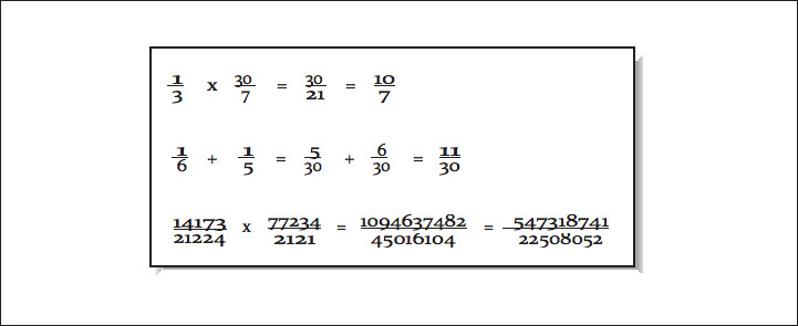
Figure 3.1
The limitation that occurs when using rational numbers to represent real numbers is that the size of the numerators and denominators tends to grow. For each addition, a common denominator must be found. To keep the numbers from becoming extremely large, during each operation, it is important to nd the greatest common divisor (GCD) to reduce fractions to their most compact representation. When the values grow and there are no common divisors, either the large integer values must be stored using dynamic memory or some form of approximation must be used, thus losing the primary advantage of rational numbers.
For mathematical packages such as Maple or Mathematica that need to produce exact results on smaller data sets, the use of rational numbers to represent real numbers is at times a useful technique. The performance and storage cost is less signicant than the need to produce exact results in some instances.
3.3.1.3 Fixed Point
If the desired number of decimal places is known in advance, it's possible to use xed-point representation.
Using this technique, each real number is stored as a scaled integer. This solves the problem that base-10 fractions such as 0.1 or 0.01 cannot be perfectly represented as a base-2 fraction. If you multiply 110.77 by 100 and store it as a scaled integer 11077, you can perfectly represent the base-10 fractional part (0.77).
This approach can be used for values such as money, where the number of digits past the decimal point is small and known.
However, just because all numbers can be accurately represented it doesn't mean there are not errors with this format. When multiplying a xed-point number by a fraction, you get digits that can't be represented in a xed-point format, so some form of rounding must be used. For example, if you have $125.87 in the bank at 4% interest, your interest amount would be $5.0348. However, because your bank balance only has two digits of accuracy, they only give you $5.03, resulting in a balance of $130.90. Of course you probably have heard many stories of programmers getting rich depositing many of the remaining 0.0048 amounts into their own account. My guess is that banks have probably gured that one out by now, and the bank keeps the money for itself. But it does make one wonder if they round or truncate in this type of calculation.6
6Perhaps banks round this instead of truncating, knowing that they will always make it up in teller machine fees.
3.3.1.4 Mantissa/Exponent
The oating-point format that is most prevalent in high performance computing is a variation on scientic notation. In scientic notation the real number is represented using a mantissa, base, and exponent: 6.02 ×
1023.The mantissa typically has some xed number of places of accuracy. The mantissa can be represented in base 2, base 16, or BCD. There is generally a limited range of exponents, and the exponent can be expressed as a power of 2, 10, or 16.
The primary advantage of this representation is that it provides a wide overall range of values while using a xed-length storage representation. The primary limitation of this format is that the dierence between two successive values is not uniform. For example, assume that you can represent three base-10 digits, and your exponent can range from 10 to 10. For numbers close to zero, the distance between successive numbers is very small. For the number 1.72 × 10⁻¹⁰, the next larger number is 1.73 × 10⁻¹⁰. The distance between these two close small numbers is 0.000000000001. For the number 6.33 × 10¹⁰, the next larger number is 6.34 × 10¹⁰. The distance between these close large numbers is 100 million.
In Figure 3.2 (Figure 4-2: Distance between successive oating-point numbers), we use two base-2 digits with an exponent ranging from 1 to 1.
Figure 4-2: Distance between successive oating-point numbers
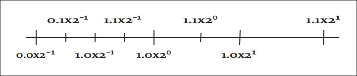
Figure 3.2
There are multiple equivalent representations of a number when using scientic notation:
6.00 × 10⁵
0.60 × 10⁶
0.06 × 10⁷
By convention, we shift the mantissa (adjust the exponent) until there is exactly one nonzero digit to the left of the decimal point. When a number is expressed this way, it is said to be normalized. In the above list, only 6.00 × 10⁵ is normalized. Figure 3.3 (Figure 4-3: Normalized oating-point numbers) shows how some of the oating-point numbers from Figure 3.2 (Figure 4-2: Distance between successive oating-point numbers) are not normalized.
While the mantissa/exponent has been the dominant oating-point approach for high performance computing, there were a wide variety of specic formats in use by computer vendors. Historically, each computer vendor had their own particular format for oating-point numbers. Because of this, a program executed on several dierent brands of computer would generally produce dierent answers. This invariably led to heated discussions about which system provided the right answer and which system(s) were generating meaningless results.7
7Interestingly, there was an easy answer to the question for many programmers. Generally they trusted the results from the computer they used to debug the code and dismissed the results from other computers as garbage.
Figure 4-3: Normalized oating-point numbers
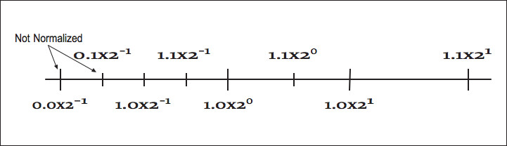
Figure 3.3
When storing oating-point numbers in digital computers, typically the mantissa is normalized, and then the mantissa and exponent are converted to base-2 and packed into a 32- or 64-bit word. If more bits were allocated to the exponent, the overall range of the format would be increased, and the number of digits of accuracy would be decreased. Also the base of the exponent could be base-2 or base-16. Using 16 as the base for the exponent increases the overall range of exponents, but because normalization must occur on four-bit boundaries, the available digits of accuracy are reduced on the average. Later we will see how the IEEE 754 standard for oating-point format represents numbers.
3.4 Eects of Floating-Point Representation8
3.4.1 Eects of Floating-Point Representation
One problem with the mantissa/base/exponent representation is that not all base-10 numbers can be expressed perfectly as a base-2 number. For example, 1/2 and 0.25 can be represented perfectly as base-2 values, while 1/3 and 0.1 produce innitely repeating base-2 decimals. These values must be rounded to be stored in the oating-point format. With sucient digits of precision, this generally is not a problem for computations. However, it does lead to some anomalies where algebraic rules do not appear to apply.
Consider the following example:
REAL*4 X,Y
X = 0.1
Y = 0
DO I=1,10
Y = Y + X
ENDDO
IF ( Y .EQ. 1.0 ) THEN
PRINT *,'Algebra is truth'
ELSE
8This content is available online at <http://cnx.org/content/m32755/1.1/>.
PRINT *,'Not here'
ENDIF
PRINT *,1.0-Y
END
At rst glance, this appears simple enough. Mathematics tells us ten times 0.1 should be one. Unfortunately, because 0.1 cannot be represented exactly as a base-2 decimal, it must be rounded. It ends up being rounded down to the last bit. When ten of these slightly smaller numbers are added together, it does not quite add up to 1.0. When X and Y are REAL*4, the dierence is about 10-7, and when they are REAL*8, the dierence is about 10-16.
One possible method for comparing computed values to constants is to subtract the values and test to see how close the two values become. For example, one can rewrite the test in the above code to be:
IF ( ABS(1.0-Y).LT. 1E-6) THEN
PRINT *,'Close enough for government work'
ELSE
PRINT *,'Not even close'
ENDIF
The type of the variables in question and the expected error in the computation that produces Y determines the appropriate value used to declare that two values are close enough to be declared equal.
Another area where inexact representation becomes a problem is the fact that algebraic inverses do not hold with all oating-point numbers. For example, using REAL*4, the value (1.0/X) * X does not evaluate to 1.0 for 135 values of X from one to 1000. This can be a problem when computing the inverse of a matrix using LU-decomposition. LU-decomposition repeatedly does division, multiplication, addition, and subtraction. If you do the straightforward LU-decomposition on a matrix with integer coecients that has an integer solution, there is a pretty good chance you won't get the exact solution when you run your algorithm.
Discussing techniques for improving the accuracy of matrix inverse computation is best left to a numerical analysis text.
3.5 More Algebra That Doesn't Work9
3.5.1 More Algebra That Doesn't Work
While the examples in the proceeding section focused on the limitations of multiplication and division, addition and subtraction are not, by any means, perfect. Because of the limitation of the number of digits of precision, certain additions or subtractions have no eect. Consider the following example using REAL*4 with 7 digits of precision:
X = 1.25E8
Y = X + 7.5E-3
IF ( X.EQ.Y ) THEN
PRINT *,'Am I nuts or what?'
9This content is available online at <http://cnx.org/content/m32754/1.1/>.
ENDIF
While both of these numbers are precisely representable in oating-point, adding them is problematic. Prior to adding these numbers together, their decimal points must be aligned as in Figure 3.4 (Figure 4-4: Loss of accuracy while aligning decimal points).
Figure 4-4: Loss of accuracy while aligning decimal points

Figure 3.4
Unfortunately, while we have computed the exact result, it cannot t back into a REAL*4 variable (7 digits of accuracy) without truncating the 0.0075. So after the addition, the value in Y is exactly 1.25E8.
Even sadder, the addition could be performed millions of times, and the value for Y would still be 1.25E8.
Because of the limitation on precision, not all algebraic laws apply all the time. For instance, the answer you obtain from X+Y will be the same as Y+X, as per the commutative law for addition. Whichever operand you pick rst, the operation yields the same result; they are mathematically equivalent. It also means that you can choose either of the following two forms and get the same answer:
(X + Y) + Z
(Y + X) + Z
However, this is not equivalent:
(Y + Z) + X
The third version isn't equivalent to the rst two because the order of the calculations has changed. Again, the rearrangement is equivalent algebraically, but not computationally. By changing the order of the calculations, we have taken advantage of the associativity of the operations; we have made an associative transformation of the original code.
To understand why the order of the calculations matters, imagine that your computer can perform arithmetic signicant to only ve decimal places.
Also assume that the values of X, Y, and Z are .00005, .00005, and 1.0000, respectively. This means that:
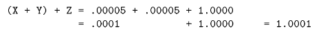
but:
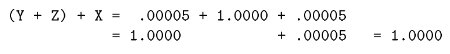
The two versions give slightly dierent answers. When adding Y+Z+X, the sum of the smaller numbers was insignicant when added to the larger number. But when computing X+Y+Z, we add the two small numbers rst, and their combined sum is large enough to inuence the nal answer. For this reason, compilers that rearrange operations for the sake of performance generally only do so after the user has requested optimizations beyond the defaults.
For these reasons, the FORTRAN language is very strict about the exact order of evaluation of expressions. To be compliant, the compiler must ensure that the operations occur exactly as you express them.10
For Kernighan and Ritchie C, the operator precedence rules are dierent. Although the precedences between operators are honored (i.e., * comes before +, and evaluation generally occurs left to right for operators of equal precedence), the compiler is allowed to treat a few commutative operations (+, *, &, and |) as if they were fully associative, even if they are parenthesized. For instance, you might tell the C compiler:
a = x + (y + z);
However, the C compiler is free to ignore you, and combine X, Y, and Z in any order it pleases.
Now armed with this knowledge, view the following harmless-looking code segment:
REAL*4 SUM,A(1000000)
SUM = 0.0
DO I=1,1000000
SUM = SUM + A(I)
ENDDO
Begins to look like a nightmare waiting to happen. The accuracy of this sum depends of the relative magnitudes and order of the values in the array A. If we sort the array from smallest to largest and then perform the additions, we have a more accurate value. There are other algorithms for computing the sum of an array that reduce the error without requiring a full sort of the data. Consult a good textbook on numerical analysis for the details on these algorithms.
If the range of magnitudes of the values in the array is relatively small, the straight- forward computation of the sum is probably sucient.
100ften even if you didn't mean it.
3.6 Improving Accuracy Using Guard Digits11
3.6.1 Improving Accuracy Using Guard Digits
In this section we explore a technique to improve the precision of oating-point computations without using additional storage space for the oating-point numbers.
Consider the following example of a base-10 system with ve digits of accuracy performing the following subtraction:
10.001 - 9.9993 = 0.0017
All of these values can be perfectly represented using our oating-point format. However, if we only have ve digits of precision available while aligning the decimal points during the computation, the results end up with signicant error as shown in Figure 3.5 (Figure 4-5: Need for guard digits ).
Figure 4-5: Need for guard digits

Figure 3.5
To perform this computation and round it correctly, we do not need to increase the number of signicant digits for stored values. We do, however, need additional digits of precision while performing the computation.
The solution is to add extra guard digits which are maintained during the interim steps of the computation. In our case, if we maintained six digits of accuracy while aligning operands, and rounded before normalizing and assigning the nal value, we would get the proper result. The guard digits only need to be present as part of the oating-point execution unit in the CPU. It is not necessary to add guard digits to the registers or to the values stored in memory.
It is not necessary to have an extremely large number of guard digits. At some point, the dierence in the magnitude between the operands becomes so great that lost digits do not aect the addition or rounding results.
3.7 History of IEEE Floating-Point Format12
3.7.1 History of IEEE Floating-Point Format
Prior to the RISC microprocessor revolution, each vendor had their own oating- point formats based on their designers' views of the relative importance of range versus accuracy and speed versus accuracy. It was not uncommon for one vendor to carefully analyze the limitations of another vendor's oating-point format and use this information to convince users that theirs was the only accurate oating- point implementation.
In reality none of the formats was perfect. The formats were simply imperfect in dierent ways.
11This content is available online at <http://cnx.org/content/m32744/1.1/>.
12This content is available online at <http://cnx.org/content/m32770/1.1/>.
During the 1980s the Institute for Electrical and Electronics Engineers (IEEE) produced a standard for the oating-point format. The title of the standard is IEEE 754-1985 Standard for Binary Floating-Point Arithmetic. This standard provided the precise denition of a oating-point format and described the operations on oating-point values.
Because IEEE 754 was developed after a variety of oating-point formats had been in use for quite some time, the IEEE 754 working group had the benet of examining the existing oating-point designs and taking the strong points, and avoiding the mistakes in existing designs. The IEEE 754 specication had its beginnings in the design of the Intel i8087 oating-point coprocessor. The i8087 oating-point format improved on the DEC VAX oating-point format by adding a number of signicant features.
The near universal adoption of IEEE 754 oating-point format has occurred over a 10-year time period.
The high performance computing vendors of the mid 1980s (Cray IBM, DEC, and Control Data) had their own proprietary oating-point formats that they had to continue supporting because of their installed user base. They really had no choice but to continue to support their existing formats. In the mid to late 1980s the primary systems that supported the IEEE format were RISC workstations and some coprocessors for microprocessors. Because the designers of these systems had no need to protect a proprietary oating-point format, they readily adopted the IEEE format. As RISC processors moved from general-purpose integer computing to high performance oating-point computing, the CPU designers found ways to make IEEE oating-point operations operate very quickly. In 10 years, the IEEE 754 has gone from a standard for oating-point coprocessors to the dominant oating-point standard for all computers. Because of this standard, we, the users, are the beneciaries of a portable oating-point environment.
3.7.2 IEEE Floating-Point Standard
The IEEE 754 standard specied a number of dierent details of oating-point operations, including:
• Storage formats
• Precise specications of the results of operations
• Special values
• Specied runtime behavior on illegal operations
Specifying the oating-point format to this level of detail insures that when a computer system is compliant with the standard, users can expect repeatable execution from one hardware platform to another when operations are executed in the same order.
3.7.3 IEEE Storage Format
The two most common IEEE oating-point formats in use are 32- and 64-bit numbers. Table 3.1: Table 4-1: Parameters of IEEE 32- and 64-Bit Formats gives the general parameters of these data types.
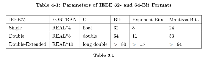
In FORTRAN, the 32-bit format is usually called REAL, and the 64-bit format is usually called DOUBLE.
However, some FORTRAN compilers double the sizes for these data types. For that reason, it is safest to declare your FORTRAN variables as REAL*4 or REAL*8. The double-extended format is not as well supported in compilers and hardware as the single- and double-precision formats. The bit arrangement for the single and double formats are shown in Figure 3.6 (Figure 4-6: IEEE754 oating-point formats).
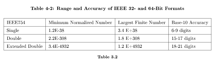
Based on the storage layouts in Table 3.1: Table 4-1: Parameters of IEEE 32- and 64-Bit Formats, we can derive the ranges and accuracy of these formats, as shown in Table 3.2: Table 4-2: Range and Accuracy of IEEE 32- and 64-Bit Formats.
Figure 4-6: IEEE754 oating-point formats
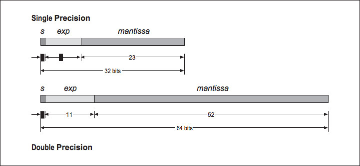
Figure 3.6
3.7.3.1 Converting from Base-10 to IEEE Internal Format
We now examine how a 32-bit oating-point number is stored. The high-order bit is the sign of the number.
Numbers are stored in a sign-magnitude format (i.e., not 2's - complement). The exponent is stored in the 8-bit eld biased by adding 127 to the exponent. This results in an exponent ranging from -126 through +127.
The mantissa is converted into base-2 and normalized so that there is one nonzero digit to the left of the binary place, adjusting the exponent as necessary. The digits to the right of the binary point are then stored in the low-order 23 bits of the word. Because all numbers are normalized, there is no need to store the leading 1.
This gives a free extra bit of precision. Because this bit is dropped, it's no longer proper to refer to the stored value as the mantissa. In IEEE parlance, this mantissa minus its leading digit is called the signicand.
Figure 3.7 (Figure 4-7: Converting from base-10 to IEEE 32-bit format) shows an example conversion from base-10 to IEEE 32-bit format.
Figure 4-7: Converting from base-10 to IEEE 32-bit format
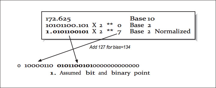
Figure 3.7
The 64-bit format is similar, except the exponent is 11 bits long, biased by adding 1023 to the exponent, and the signicand is 54 bits long.
3.8 IEEE Operations13
3.8.1 IEEE Operations
The IEEE standard species how computations are to be performed on oating- point values on the following operations:
• Addition
• Subtraction
• Multiplication
• Division
• Square root
• Remainder (modulo)
• Conversion to/from integer
• Conversion to/from printed base-10
These operations are specied in a machine-independent manner, giving exibility to the CPU designers to implement the operations as eciently as possible while maintaining compliance with the standard. During operations, the IEEE standard requires the maintenance of two guard digits and a sticky bit for intermediate values. The guard digits above and the sticky bit are used to indicate if any of the bits beyond the second guard digit is nonzero.
13This content is available online at <http://cnx.org/content/m32756/1.1/>.
Figure 4-8: Computation using guard and sticky bits
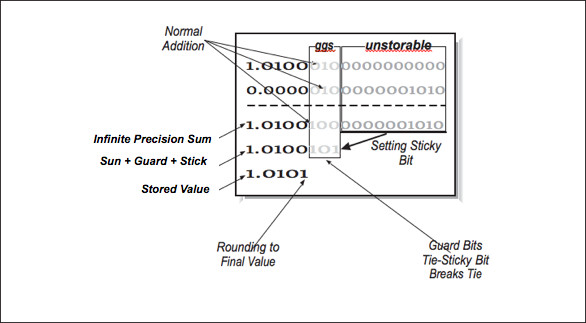
Figure 3.8
In Figure 3.8 (Figure 4-8: Computation using guard and sticky bits), we have ve bits of normal precision, two guard digits, and a sticky bit. Guard bits simply operate as normal bits as if the signicand were bits. Guard bits participate in rounding as the extended operands are added. The sticky