Chapter 4
Understanding Parallelism
4.1 Introduction1
4.1.1 Understanding Parallelism
In a sense, we have been talking about parallelism from the beginning of the book. Instead of calling it parallelism, we have been using words like pipelined, superscalar, and compiler exibility. As we move into programming on multiprocessors, we must increase our understanding of parallelism in order to understand how to eectively program these systems. In short, as we gain more parallel resources, we need to nd more parallelism in our code.
When we talk of parallelism, we need to understand the concept of granularity. The granularity of parallelism indicates the size of the computations that are being performed at the same time between synchronizations. Some examples of parallelism in order of increasing grain size are:
• When performing a 32-bit integer addition, using a carry lookahead adder, you can partially add bits 0 and 1 at the same time as bits 2 and 3.
• On a pipelined processor, while decoding one instruction, you can fetch the next instruction.
• On a two-way superscalar processor, you can execute any combination of an integer and a oating-point instruction in a single cycle.
• On a multiprocessor, you can divide the iterations of a loop among the four processors of the system.
• You can split a large array across four workstations attached to a network. Each workstation can operate on its local information and then exchange boundary values at the end of each time step.
In this chapter, we start at instruction-level parallelism (pipelined and superscalar) and move toward thread-level parallelism, which is what we need for multiprocessor systems. It is important to note that the dierent levels of parallelism are generally not in conict. Increasing thread parallelism at a coarser grain size often exposes more ne-grained parallelism.
The following is a loop that has plenty of parallelism:
DO I=1,16000
A(I) = B(I) * 3.14159
ENDDO
1This content is available online at <http://cnx.org/content/m32775/1.1/>.
We have expressed the loop in a way that would imply that A(1) must be computed rst, followed by A(2), and so on. However, once the loop was completed, it would not have mattered if A(16000), were computed rst followed by A(15999), and so on. The loop could have computed the even values of I and then computed the odd values of I. It would not even make a dierence if all 16,000 of the iterations were computed simultaneously using a 16,000-way superscalar processor.2 If the compiler has exibility in the order in which it can execute the instructions that make up your program, it can execute those instructions simultaneously when parallel hardware is available.
One technique that computer scientists use to formally analyze the potential parallelism in an algorithm is to characterize how quickly it would execute with an innite-way superscalar processor.
Not all loops contain as much parallelism as this simple loop. We need to identify the things that limit the parallelism in our codes and remove them whenever possible. In previous chapters we have already looked at removing clutter and rewriting loops to simplify the body of the loop.
This chapter also supplements Chapter 5, What a Compiler Does, in many ways. We looked at the mechanics of compiling code, all of which apply here, but we didn't answer all of the whys. Basic block analysis techniques form the basis for the work the compiler does when looking for more parallelism. Looking at two pieces of data, instructions, or data and instructions, a modern compiler asks the question, Do these things depend on each other? The three possible answers are yes, no, and we don't know. The third answer is eectively the same as a yes, because a compiler has to be conservative whenever it is unsure whether it is safe to tweak the ordering of instructions.
Helping the compiler recognize parallelism is one of the basic approaches specialists take in tuning code.
A slight rewording of a loop or some supplementary information supplied to the compiler can change a we don't know answer into an opportunity for parallelism. To be certain, there are other facets to tuning as well, such as optimizing memory access patterns so that they best suit the hardware, or recasting an algorithm. And there is no single best approach to every problem; any tuning eort has to be a combination of techniques.
4.2 Dependencies3
4.2.1 Dependencies
Imagine a symphony orchestra where each musician plays without regard to the conductor or the other musicians. At the rst tap of the conductor's baton, each musician goes through all of his or her sheet music. Some nish far ahead of others, leave the stage, and go home. The cacophony wouldn't resemble music (come to think of it, it would resemble experimental jazz) because it would be totally uncoordinated.
Of course this isn't how music is played. A computer program, like a musical piece, is woven on a fabric that unfolds in time (though perhaps woven more loosely). Certain things must happen before or along with others, and there is a rate to the whole process.
With computer programs, whenever event A must occur before event B can, we say that B is dependent on A. We call the relationship between them a dependency. Sometimes dependencies exist because of calculations or memory operations; we call these data dependencies. Other times, we are waiting for a branch or do-loop exit to take place; this is called a control dependency. Each is present in every program to varying degrees. The goal is to eliminate as many dependencies as possible. Rearranging a program so that two chunks of the computation are less dependent exposes parallelism, or opportunities to do several things at once.
2Interestingly, this is not as far-fetched as it might seem. On a single instruction multiple data (SIMD) computer such as the Connection CM-2 with 16,384 processors, it would take three instruction cycles to process this entire loop. See Chapter 12, Large-Scale Parallel Computing, for more details on this type of architecture.
3This content is available online at <http://cnx.org/content/m32777/1.1/>.
4.2.1.1 Control Dependencies
Just as variable assignments can depend on other assignments, a variable's value can also depend on the ow of control within the program. For instance, an assignment within an if-statement can occur only if the conditional evaluates to true. The same can be said of an assignment within a loop. If the loop is never entered, no statements inside the loop are executed.
When calculations occur as a consequence of the ow of control, we say there is a control dependency, as in the code below and shown graphically in Figure 4.1 (Figure 9-1: Control dependency). The assignment located inside the block-if may or may not be executed, depending on the outcome of the test X .NE. 0.
In other words, the value of Y depends on the ow of control in the code around it. Again, this may sound to you like a concern for compiler designers, not programmers, and that's mostly true. But there are times when you might want to move control-dependent instructions around to get expensive calculations out of the way (provided your compiler isn't smart enough to do it for you). For example, say that Figure 4.2 (Figure 9-2: A little section of your program) represents a little section of your program. Flow of control enters at the top and goes through two branch decisions. Furthermore, say that there is a square root operation at the entry point, and that the ow of control almost always goes from the top, down to the leg containing the statement A=0.0. This means that the results of the calculation A=SQRT(B) are almost always discarded because A gets a new value of 0.0 each time through. A square root operation is always expensive because it takes a lot of time to execute. The trouble is that you can't just get rid of it; occasionally it's needed.
However, you could move it out of the way and continue to observe the control dependencies by making
two copies of the square root operation along the less traveled branches, as shown in Figure 4.3 (Figure 9-3: Expensive operation moved so that it's rarely executed). This way the SQRT would execute only along those paths where it was actually needed.
Figure 9-1: Control dependency
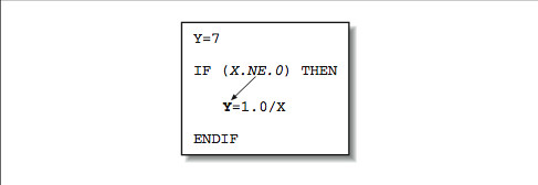
Figure 4.1
Figure 9-2: A little section of your program
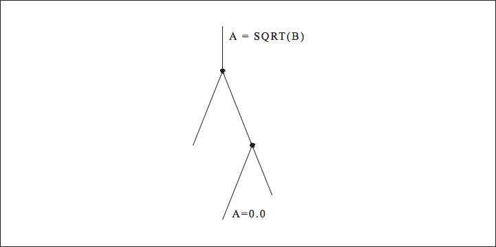
Figure 4.2
This kind of instruction scheduling will be appearing in compilers (and even hardware) more and more as time goes on. A variation on this technique is to calculate results that might be needed at times when there is a gap in the instruction stream (because of dependencies), thus using some spare cycles that might otherwise be wasted.
Figure 9-3: Expensive operation moved so that it's rarely executed
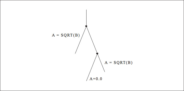
Figure 4.3
4.2.1.2 Data Dependencies
A calculation that is in some way bound to a previous calculation is said to be data dependent upon that calculation. In the code below, the value of B is data dependent on the value of A. That's because you can't calculate B until the value of A is available:
A = X + Y + COS(Z)
B = A * C
This dependency is easy to recognize, but others are not so simple. At other times, you must be careful not to rewrite a variable with a new value before every other computation has nished using the old value. We can group all data dependencies into three categories: (1) ow dependencies, (2) antidependencies, and (3) output dependencies. Figure 4.4 (Figure 9-4: Types of data dependencies) contains some simple examples to demonstrate each type of dependency. In each example, we use an arrow that starts at the source of the dependency and ends at the statement that must be delayed by the dependency. The key problem in each of these dependencies is that the second statement can't execute until the rst has completed. Obviously in the particular output dependency example, the rst computation is dead code and can be eliminated unless there is some intervening code that needs the values. There are other techniques to eliminate either output or antidependencies. The following example contains a ow dependency followed by an output dependency.
Figure 9-4: Types of data dependencies
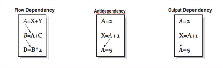
Figure 4.4
X = A / B
Y = X + 2.0
X = D - E
While we can't eliminate the ow dependency, the output dependency can be eliminated by using a scratch variable:
Xtemp = A/B
Y = Xtemp + 2.0
X = D - E
As the number of statements and the interactions between those statements increase, we need a better way to identify and process these dependencies. Figure 4.5 (Figure 9-5: Multiple dependencies) shows four statements with four dependencies.
Figure 9-5: Multiple dependencies
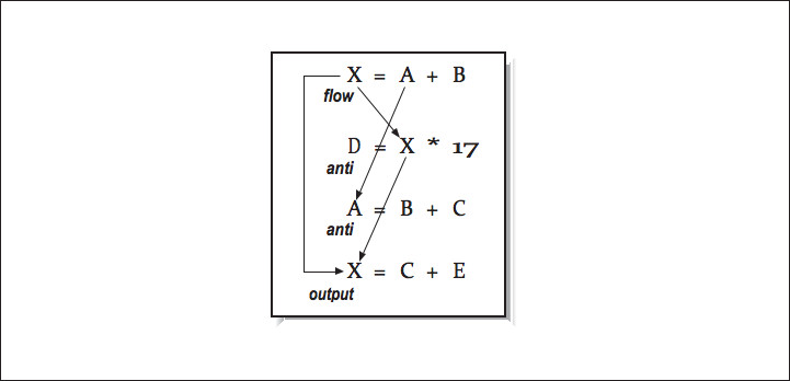
Figure 4.5
None of the second through fourth instructions can be started before the rst instruction completes.
4.2.1.3 Forming a DAG
One method for analyzing a sequence of instructions is to organize it into a directed acyclic graph (DAG).4
Like the instructions it represents, a DAG describes all of the calculations and relationships between variables.
The data ow within a DAG proceeds in one direction; most often a DAG is constructed from top to bottom.
Identiers and constants are placed at the leaf nodes the ones on the top. Operations, possibly with variable names attached, make up the internal nodes. Variables appear in their nal states at the bottom.
The DAG's edges order the relationships between the variables and operations within it. All data ow proceeds from top to bottom.
To construct a DAG, the compiler takes each intermediate language tuple and maps it onto one or more nodes. For instance, those tuples that represent binary operations, such as addition (X=A+B), form a portion of the DAG with two inputs (A and B) bound together by an operation (+). The result of the operation may feed into yet other operations within the basic block (and the DAG) as shown in Figure 4.6 (Figure 9-6: A trivial data ow graph).
4A graph is a collection of nodes connected by edges. By directed, we mean that the edges can only be traversed in specied directions. The word acyclic means that there are no cycles in the graph; that is, you can't loop anywhere within it.
Figure 9-6: A trivial data ow graph
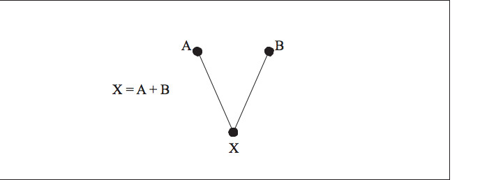
Figure 4.6
For a basic block of code, we build our DAG in the order of the instructions. The DAG for the previous four instructions is shown in Figure 4.7 (Figure 9-7: A more complex data ow graph). This particular example has many dependencies, so there is not much opportunity for parallelism. Figure 4.8 (Figure 9-8: Extracting parallelism from a DAG) shows a more straightforward example shows how constructing a DAG can identify parallelism.
From this DAG, we can determine that instructions 1 and 2 can be executed in parallel. Because we see the computations that operate on the values A and B while processing instruction 4, we can eliminate a common subexpression during the construction of the DAG. If we can determine that Z is the only variable that is used outside this small block of code, we can assume the Y computation is dead code.
Figure 9-7: A more complex data ow graph
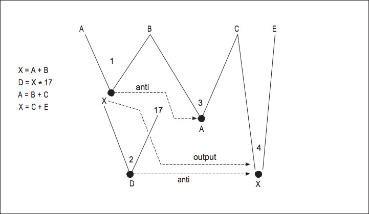
Figure 4.7
By constructing the DAG, we take a sequence of instructions and determine which must be executed in a particular order and which can be executed in parallel. This type of data ow analysis is very important in the codegeneration phase on super-scalar processors. We have introduced the concept of dependencies and how to use data ow to nd opportunities for parallelism in code sequences within a basic block. We can also use data ow analysis to identify dependencies, opportunities for parallelism, and dead code between basic blocks.
4.2.1.4 Uses and Denitions
As the DAG is constructed, the compiler can make lists of variable uses and denitions, as well as other information, and apply these to global optimizations across many basic blocks taken together. Looking at the DAG in Figure 4.8 (Figure 9-8: Extracting parallelism from a DAG), we can see that the variables dened are Z, Y, X, C, and D, and the variables used are A and B. Considering many basic blocks at once, we can say how far a particular variable denition reaches where its value can be seen. From this we can recognize situations where calculations are being discarded, where two uses of a given variable are completely independent, or where we can overwrite register-resident values without saving them back to memory. We call this investigation data ow analysis.
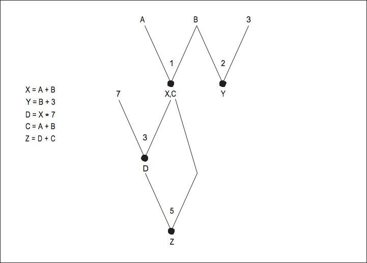
Figure 4.8
To illustrate, suppose that we have the ow graph in Figure 4.9 (Figure 9-9: Flow graph for data ow analysis). Beside each basic block we've listed the variables it uses and the variables it denes. What can data ow analysis tell us?
Notice that a value for A is dened in block X but only used in block Y. That means that A is dead upon exit from block Y or immediately upon taking the right-hand branch leaving X; none of the other basic blocks uses the value of A. That tells us that any associated resources, such as a register, can be freed for other uses.Looking at Figure 4.9 (Figure 9-9: Flow graph for data ow analysis) we can see that D is dened in basic block X, but never used. This means that the calculations dening D can be discarded.
Something interesting is happening with the variable G. Blocks X and W both use it, but if you look closely you'll see that the two uses are distinct from one another, meaning that they can be treated as two independent variables.
A compiler featuring advanced instruction scheduling techniques might notice that W is the only block that uses the value for E, and so move the calculations dening E out of block Y and into W, where they are needed.
Figure 9-9: Flow graph for data ow analysis
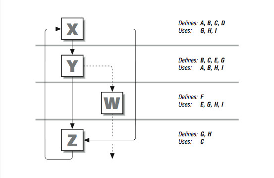
Figure 4.9
In addition to gathering data about variables, the compiler can also keep information about subexpressions. Examining both together, it can recognize cases where redundant calculations are being made (across basic blocks), and substitute previously computed values in their place. If, for instance, the expression H*I appears in blocks X, Y, and W, it could be calculated just once in block X and propagated to the others that use it.
4.3 Loops5
4.3.1 Loops
Loops are the center of activity for many applications, so there is often a high payback for simplifying or moving calculations outside, into the computational suburbs. Early compilers for parallel architectures used pattern matching to identify the bounds of their loops. This limitation meant that a hand-constructed loop using if-statements and goto-statements would not be correctly identied as a loop. Because modern compilers use data ow graphs, it's practical to identify loops as a particular subset of nodes in the ow graph.
To a data ow graph, a hand constructed loop looks the same as a compiler-generated loop. Optimizations can therefore be applied to either type of loop.
5This content is available online at <http://cnx.org/content/m32784/1.1/>.
Once we have identied the loops, we can apply the same kinds of data-ow analysis we applied above.
Among the things we are looking for are calculations that are unchanging within the loop and variables that change in a predictable (linear) fashion from iteration to iteration.
How does the compiler identify a loop in the ow graph? Fundamentally, two conditions have to be met:
• A given node has to dominate all other nodes within the suspected loop. This means that all paths to any node in the loop have to pass through one particular node, the dominator. The dominator node forms the header at the top of the loop.
• There has to be a cycle in the graph. Given a dominator, if we can nd a path back to it from one of the nodes it dominates, we have a loop. This path back is known as the back edge of the loop.
The ow graph in Figure 4.10 (Figure 9-10: Flowgraph with a loop in it) contains one loop and one red herring. You can see that node B dominates every node below it in the subset of the ow graph. That satises Condition 1 and makes it a candidate for a loop header. There is a path from E to B, and B dominates E, so that makes it a back edge, satisfying Condition 2. Therefore, the nodes B, C, D, and E form a loop. The loop goes through an array of linked list start pointers and traverses the lists to determine the total number of nodes in all lists. Letters to the extreme right correspond to the basic block numbers in the ow graph.
Figure 9-10: Flowgraph with a loop in it
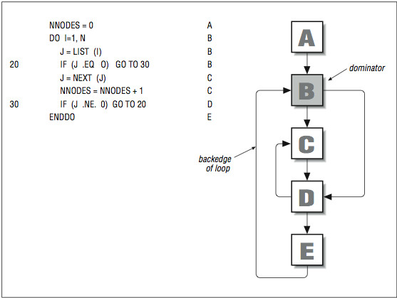
Figure 4.10
At rst glance, it appears that the nodes C and D form a loop too. The problem is that C doesn't dominate D (and vice versa), because entry to either can be made from B, so condition 1 isn't satised. Generally, the ow graphs that come from code segments written with even the weakest appreciation for a structured design oer better loop candidates.
After identifying a loop, the compiler can concentrate on that portion of the ow graph, looking for instructions to remove or push to the outside. Certain types of subexpressions, such as those found in array index expressions, can be simplied if they change in a predictable fashion from one iteration to the next.
In the continuing quest for parallelism, loops are generally our best sources for large amounts of parallelism. However, loops also provide new opportunities for those parallelism-killing dependencies.
4.4 Loop-Carried Dependencies 6
4.4.1 Loop-Carried Dependencies
The notion of data dependence is particularly important when we look at loops, the hub of activity inside numerical applications. A well-designed loop can produce millions of operations that can all be performed in parallel. However, a single misplaced dependency in the loop can force it all to be run in serial. So the stakes are higher when looking for dependencies in loops.
Some constructs are completely independent, right out of the box. The question we want to ask is Can two dierent iterations execute at the same time, or is there a data dependency between them? Consider the following loop:
DO I=1,N
A(I) = A(I) + B(I)
ENDDO
For any two values of I and K, can we calculate the value of A(I) and A(K) at the same time? Below, we have manually unrolled several iterations of the previous loop, so they can be executed together:
A(I) = A(I) + B(I)
A(I+1) = A(I+1) + B(I+1)
A(I+2) = A(I+2) + B(I+2)
You can see that none of the results are used as an operand for another calculation. For instance, the calculation for A(I+1) can occur at the same time as the calculation for A(I) because the calculations are independent; you don't need the results of the rst to determine the second. In fact, mixing up the order of the calculations won't change the results in the least. Relaxing the serial order imposed on these calculations makes it possible to execute this loop very quickly on parallel hardware.
4.4.1.1 Flow Dependencies
For comparison, look at the next code fragment:
6This content is available online at <http://cnx.org/content/m32782/1.1/>.
DO I=2,N
A(I) = A(I-1) + B(I)
ENDDO
This loop has the regularity of the previous example, but one of the subscripts is changed. Again, it's useful to manually unroll the loop and look at several iterations together:
A(I) = A(I-1) + B(I)
A(I+1) = A(I) + B(I+1)
A(I+2) = A(I+1) + B(I+2)
In this case, there is a dependency problem. The value of A(I+1) depends on the value of A(I), the value of A(I+2) depends on A(I+1), and so on; every iteration depends on the result of a previous one. Dependencies that extend back to a previous calculation and perhaps a previous iteration (like this one), are loop carried ow dependencies or backward dependencies. You often see such dependencies in applications that perform Gaussian elimination on certain types of matrices, or numerical solutions to systems of dierential equations.
However, it is impossible to run such a loop in parallel (as written); the processor must wait for intermediate results before it can proceed.
In some cases, ow dependencies are impossible to x; calculations are so dependent upon one another that we have no choice but to wait for previous ones to complete. Other times, dependencies are a function of the way the calculations are expressed. For instance, the loop above can be changed to reduce the dependency. By replicating some of the arithmetic, we can make it so that the second and third iterations depend on the rst, but not on one another. The operation count goes up we have an extra addition that we didn't have before but we have reduced the dependency between iterations:
DO I=2,N,2
A(I)
= A(I-1) + B(I)
A(I+1) = A(I-1) + B(I) + B(I+1)
ENDDO
The speed increase on a workstation won't be great (most machines run the recast loop more slowly).
However, some parallel computers can trade o additional calculations for reduced dependency and chalk up a net win.
4.4.1.2 Antidependencies
It's a dierent story when there is a loop-carried antidependency, as in the code below:
DO I=1,N
A(I) = B(I) * E
B(I) = A(I+2) * C
ENDDO
In this loop, there is an antidependency between the variable A(I) and the variable A(I+2). That is, you must be sure that the instruction that uses A(I+2) does so before the previous one redenes it. Clearly, this is not a problem if the loop is executed serially, but remember, we are looking for opportunities to overlap instructions. Again, it helps to pull the loop apart and look at several iterations together. We have recast the loop by making many copies of the rst statement, followed by copies of the second:
A(I) = B(I) * E
A(I+1) = B(I+1) * E
A(I+2) = B(I+2) * E
...
B(I) = A(I+2) * C ← assignment makes use of the new
B(I+1) = A(I+3) * C value of A(I+2) incorrect.
B(I+2) = A(I+4) * C
The reference to A(I+2) needs to access an old value, rather than one of the new ones being calculated.
If you perform all of the rst statement followed by all of the second statement, the answers will be wrong.
If you perform all of the second statement followed by all of the rst statement, the answers will also be wrong. In a sense, to run the iterations in parallel, you must either save the A values to use for the second statement or store all of the B value in a temporary area until the loop completes.
We can also directly unroll the loop and nd some parallelism:
1 A(I) = B(I) * E
2 B(I) = A(I+2) * C →
3 A(I+1) = B(I+1) * E | Output dependency
4 B(I+1) = A(I+3) * C |
5 A(I+2) = B(I+2) * E ←
6 B(I+2) = A(I+4) * C
Statements 14 could all be executed simultaneously. Once those statements completed execution, statements 58 could execute in parallel. Using this approach, there are sucient intervening statements between the dependent statements that we can see some parallel performance improvement from a superscalar RISC processor.
4.4.1.3 Output Dependencies
The third class of data dependencies, output dependencies, is of particular interest to users of parallel computers, particularly multiprocessors. Output dependencies involve getting the right values to the right variables when all calculations have been completed. Otherwise, an output dependency is violated. The loop below assigns new values to two elements of the vector A with each iteration:
DO I=1,N
A(I) = C(I) * 2.
A(I+2) = D(I) + E
ENDDO
As always, we won't have any problems if we execute the code sequentially. But if several iterations are performed together, and statements are reordered, then incorrect values can be assigned to the last elements of A. For example, in the naive vectorized equivalent below, A(I+2) takes the wrong value because the
assignments occur out of order:
A(I) = C(I) * 2.
A(I+1) = C(I+1) * 2.
A(I+2) = C(I+2) * 2.
A(I+2) = D(I) + E ← Output dependency violated
A(I+3) = D(I+1) + E
A(I+4) = D(I+2) + E
Whether or not you have to worry about output dependencies depends on whether you are actually parallelizing the code. Your compiler will be conscious of the danger, and will be able to generate legal code and possibly even fast code, if it's clever enough. But output dependencies occasionally become a problem for programmers.
4.4.1.4 Dependencies Within an Iteration
We have looked at dependencies that cross iteration boundaries but we haven't looked at dependencies within the same iteration. Consider the following code fragment:
DO I = 1,N
D = B(I) * 17
A(I) = D + 14
ENDDO
When we look at the loop, the variable D has a ow dependency. The second statement cannot start until the rst statement has completed. At rst glance this might appear to limit parallelism signicantly. When we look closer and manually unroll several iterations of the loop, the situation gets worse:
D = B(I) * 17
A(I) = D + 14
D = B(I+1) * 17
A(I+1) = D + 14
D = B(I+2) * 17
A(I+2) = D + 14
Now, the variable D has ow, output, and antidependencies. It looks like this loop has no hope of running in parallel. However, there is a simple solution to this problem at the cost of some extra memory space, using a technique called promoting a scalar to a vector. We dene D as an array withN elements and rewrite the code as follows:
DO I = 1,N
D(I) = B(I) * 17
A(I) = D(I) + 14
ENDDO
Now the iterations are all independent and can be run in parallel. Within each iteration, the rst statement must run before the second statement.
4.4.1.5 Reductions
The sum of an array of numbers is one example of a reduction so called because it reduces a vector to a scalar. The following loop to determine the total of the values in an array certainly looks as though it might be able to be run in parallel:
SUM = 0.0
DO I=1,N
SUM = SUM + A(I)
ENDDO
However, i