The heartbeat extension protocol consists of two message types: HeartbeatRequest message and HeartbeatResponse message and the extension protocol depends on which TLS protocol is being used as describe below:
3.1.1 When Using Reliable Transport Protocol
One side of the peer connection sends a HeartbeatRequest message to the other side. The other side of the connection should immediately send a HeartbeatResponse message. This makes one successful Heartbeat and thus, keeping connection alive – this is called ‘keep-alive’ functionality. If no response is received within a specified timeout, the TLS connection is terminated.
3.1.2 Unreliable Transport Protocol
One side of the peer connection sends HeartbeatRequest message to the other side. The other side of the connection should immediately send a HeartbeatResponse message. If no response is received within specified timeout another HeartbeatRequest message is retransmitted. If expected response is not received for specified number of retransmissions, the DTLS (Datagram Transport Layer Security) connection is terminated.
When a receiver receives a HeartbeatRequest message, the receiver should send back an exact copy of the received message in the HeartbeatResponse message. The sender verifies that the HeartbeatResponse message is same as what was originally sent. If it is same, the connection is kept alive. If the response does not contain the same message, the HeartbeatRequest message is retransmitted for a specified number of retransmissions [7].
There is a bug in the implementation of the Heartbeat reply to the received Heartbeat request message. Heartbeat reply copies the received payload to the Heartbeat response message to verify that the secured connection is still active, without checking if the payload length is same as the length of the request payload data.
The problem here is that the OpenSSL heartbeat response code does not check to make sure that the payload length field specified in the heartbeat request message matches the actual length of the payload.
If the heartbeat request payload length field is set to a value larger than the actual payload, it would result in a return of the payload followed by whatever contents are currently contained in active memory buffer, beyond the end of the payload. A heartbeat request the payload length can be set to a maximum value of 65535 bytes. Therefore the bug in the OpenSSL heartbeat response code could copy as much as 65535 bytes from the machine's memory and send it to the requestor [6].
This bug is illustrated below in “Figure 1: Memory Leak.

“Figure 1: Memory leak” shows that when the request payload data is ‘ma’ and payload length is ‘2’ then 2 bytes from source (i.e. ‘ma’) is copied to the ‘destination’ memory area. But when the request payload data is ‘ma’ and payload length falsely indicates that it is 8 bytes instead of 2, 8 bytes (i.e. ‘madadbro’) from the ‘source’ memory area to the ‘destination’ memory area. This ‘destination’ data is finally sent to the requestor, causing the memory leak that is now known as the Heartbleed bug [9].
“Figure 2: The OpenSSL code fix for the Heartbleed bug” shows the change in OpenSSL's file t1_lib.c between version 1.0.1 and OpenSSL version 1.0.1g that was made to fix the Heartbleed bug [7].
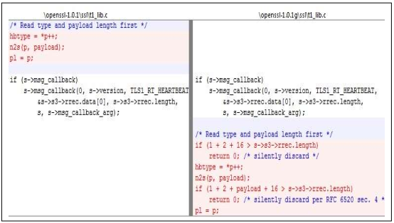
Figure 2: The OpenSSL code fix for the Heartbleed bug
This code fix has two tasks to perform:
First, it checks to determine if the length of the payload is zero or not. It simply discards the message if the payload length is 0.
The second task performed by the bug fix makes sure that the heartbeat payload length field value matches the actual length of the request payload data. If not, it discards the message.
The official notice about the bug was published by the OpenSSL group at https://www.openssl.org/news/secadv_20140407.txt and is reproduced in “Figure 3: OpenSSL Security Advisory.”
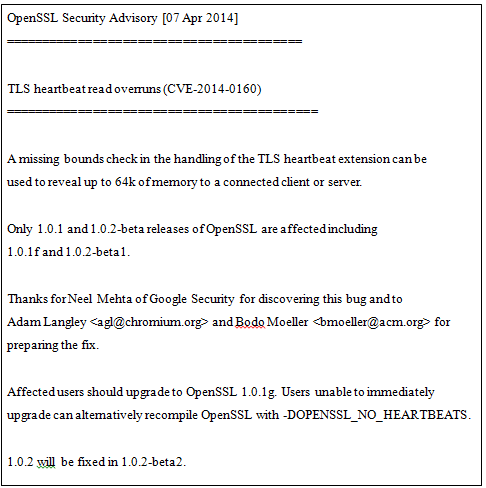
Figure 3: OpenSSL Security Advisory
By exploiting the Heartbleed vulnerability, an attacker can send a Heartbeat request message and retrieve up to 64 KB of memory from the victim's server. The contents of the retrieved memory depends on what's in memory in the server at the time, but could potentially contain usernames, passwords, session IDs or secret private keys or other sensitive information. Following figure illustrates how an attacker can exploit this vulnerability. This attack can be made multiple times without leaving any trace of it. "Figure 4: Exploiting the Heartbleed vulnerability" illustrates how an attacker can exploit the Heartbleed vulnerability.

Figure 4: Exploiting the Heartbleed vulnerability
The data used in this section comes from many different sources. The main reference source is the National Vulnerability Database (NVD), which includes Information for all Common Vulnerabilities and Exposures (CVEs). As of May 2015, there are close to 69,000 CVEs in the database. Connected to each CVE is also a list of external references to exploits, bug trackers, vendor pages, etc. Each CVE comes with some Common Vulnerability Scoring System (CVSS) metrics and parameters, which can be found in Table 1. A CVE- number is of the format CVE-Y- N, with a four number year Y, and a 4-6 number identifier N per year. Major vendors are pre-assigned ranges of CVE-numbers to be registered in the oncoming year, which means that CVE-numbers are not guaranteed to be used or to be registered in consecutive order [9].
The data from the NVD only includes the base CVSS Metric parameters seen in Table 1. In the official guide for CVSS metrics, Mell et al. (2007) describes that there are similar categories for Temporal Metrics and Environmental Metrics. The first one includes categories for Exploitability, Remediation Level, and Report Confidence. The latter includes Collateral Damage Potential, target Distribution, and Security Requirements. Part of this data is sensitive and cannot be publicly disclosed.
TABLE 1: CVSS (version 2) Base Metrics, with definitions from Mell et al. (2007)
|
Parameter |
Values |
Description |
|
CVSS Score |
0-10 [Low (0.1 -3.9), Medium (4.0 – 6.9), High (7.0 – 8.9), Critical (9.0 – 10.0)] |
This value is calculated based on the next six parameters, with a formula (Mell et al., 2007). |
|
Access Vector |
Local Adjacent Network |
The access vector (AV) determines how vulnerability can be exploited. A local attack requires physical access to the computer or a shell account. Vulnerability with Network access is also called remotely exploitable. |
|
Access Complexity |
Low Medium High |
The access complexity (AC) classifies the difficulty to exploit the vulnerability. |
|
Authentication |
None Single Multiple |
The authentication (Au) categorizes the number of times that an attacker must authenticate to a target to exploit it, but does not measure the difficulty of the authentication process itself. |
|
Confidentiality |
None Partial Complete |
The confidentiality (C) metric assorts the impact of the confidentiality, and amount of information access and disclosure. This may include partial or full access to file systems and/or database tables. |
|
Integrity |
None Partial Complete |
The integrity (I) metric categorizes the impact on the integrity of the exploited system. For example, if the remote attack is able to partially or fully modify information in the exploited system. |
|
Availability |
None Partial Complete |
The availability (A) metric categorizes the impact on the availability of the target system. Attacks that consume network bandwidth, processor cycles, memory or any other resources affect the availability of a system. |
Naive Bayes is a classification algorithm for binary (two-class) and multi-class classification problems. The technique is easiest to understand when described using binary or categorical input values [8].
It is called naive Bayes or idiot Bayes because the calculation of the probabilities for each hypothesis is simplified to make their calculation tractable. Rather than attempting to calculate the values of each attribute value P (d1, d2, d3|h), they are assumed to be conditionally independent given the target value and calculated as P (d1|h) * P (d2|H) and so on.
This is a very strong assumption that is most unlikely in real data, i.e. that the attributes do not interact. Nevertheless, the approach performs surprisingly well on data where this assumption does not hold.
3.6.1 Representation Used By Naive Bayes Models
The representation for naive Bayes is probabilities.
A list of probabilities is stored to file for a learned naive Bayes model. This includes:
3.6.2 Learn a Naive Bayes Model from Data
Learning a naive Bayes model from training data is fast.
Training is fast because only the probability of each class and the probability of each class given different input (x) values need to be calculated. No coefficients need to be fitted by optimization procedures.
3.6.3 Calculating Class Probabilities
The class probabilities are simply the frequency of instances that belong to each class divided by the total number of instances.
For example in a binary classification the probability of an instance belonging to class 1 would be calculated as:
P(class=1) = count(class=1) / (count(class=0) + count(class=1))
In the simplest case each class would have the probability of 0.5 or 50% for a binary classification problem with the same number of instances in each class.
3.6.4 Calculating Conditional Probabilities
The conditional probabilities are the frequency of each attribute value for a given class value divided by the frequency of instances with that class value.
For example, if a “weather” attribute had the values “sunny” and “rainy” and the class attribute had the class values “go-out” and “stay- home“, then the conditional probabilities of each weather value for each class value could be calculated as:
3.6.5 Make Predictions with a Naive Bayes Model
Given a naive Bayes model, you can make predictions for new data using Bayes theorem.
MAP(h) = max(P(d|h) * P(h))
Using our example above, if we had a new instance with the weather of sunny, we can calculate:
go-out = P(weather=sunny|class=go-out) * P(class=go-out)
stay-home = P(weather=sunny|class=stay-home) * P(class=stay-home)
We can choose the class that has the largest calculated value. We can turn these values into probabilities by normalizing them as follows:
P(go-out|weather=sunny) = go-out / (go-out + stay-home)
P(stay-home|weather=sunny) = stay-home / (go-out + stay-home)
If we had more input variables we could extend the above example. For example, pretend we have a “car” attribute with the values “working” and “broken“. We can multiply this probability into the equation.
For example below is the calculation for the “go-out” class label with the addition of the car input variable set to “working”:
go-out = P(weather=sunny|class=go-out) * P(car=working|class=go-out) *
P(class=go-out)
3.6.6 Gaussian Naive Bayes
Naive Bayes can be extended to real-valued attributes, most commonly by assuming a Gaussian distribution.
This extension of naive Bayes is called Gaussian Naive Bayes. Other functions can be used to estimate the distribution of the data, but the Gaussian (or Normal distribution) is the easiest to work with because you only need to estimate the mean and the standard deviation from your training data.
3.6.7 Representation for Gaussian Naive Bayes
Above, we calculated the probabilities for input values for each class using a frequency. With real-valued inputs, we can calculate the mean and standard deviation of input values (x) for each class to summarize the distribution.
This means that in addition to the probabilities for each class, we must also store the mean and standard deviations for each input variable for each class.
3.6.8 Learn a Gaussian Naive Bayes Model from Data
This is as simple as calculating the mean and standard deviation values of each input variable (x) for each class value.
mean(x) = 1/n * sum(x)
Where n is the number of instances and x are the values for an input variable in your training data.
We can calculate the standard deviation (sd) using the following equation:
standard deviation(x) = sqrt(1/n * sum(xi-mean(x)^2 ))
This is the square root of the average squared difference of each value of x from the mean value of x, where n is the number of instances, sqrt( ) is the square root function, sum( ) is the sum function, xi is a specific value of the x variable for the i’th instance and mean(x) is described above, and ^2 is the square.
3.6.9 Make Predictions with a Gaussian Naive Bayes Model
Probabilities of new x values are calculated using the Gaussian Probability Density Function (PDF).
When making predictions these parameters can be plugged into the Gaussian PDF with a new input for the variable, and in return the Gaussian PDF will provide an estimate of the probability of that new input value for that class.
pdf(x, mean, sd) = (1 / (sqrt(2 * PI) * sd)) * exp(-((x-mean^2)/(2*sd^2)))
Where pdf(x) is the Gaussian PDF, sqrt( ) is the square root, mean and sd are the mean and standard deviation calculated above, PI is the numerical constant, exp( ) is the numerical constant e or Euler’s number raised to power and x is the input value for the input variable.
We can then plug in the probabilities into the equation above to make predictions with real-valued inputs.
For example, adapting one of the above calculations with numerical values for weather and car:
go-out = P(pdf(weather)|class=go-out) * P(pdf(car)|class=go-out) * P(class=go-out)