In addition you might want to specify a stretch of the gray-scale of the image. This can be obtained first by specifying the max and min values of the displayed image (everything above is set to the max value and everything below to the min value). This is set with the Min and Max options. Additionally it is possible to adjust the image transfer function using the option ITF. Allowed values are Linear, Log and Sqrt.
You can also add a colour bar (colour wedge in PGPLOT parlance) to the image display. This is accomplished either using the draw_wedge (see below) command directly or by setting the DrawWedge option to true in your call to imag . If you want to pass options to the draw_wedge command, you can do that with the Wedge option. See below for further details.
Transforms
Finally a very useful feature of PGPLOT that is relevant both to images and also the contour plots (see below) is the concept of a transform matrix. This is a 6 element vector, T(i) which maps input pixels into display pixels so that pixel i,j is mapped to:
X(ij) = T0 + T1(i) + T2(j)
Y(ij) = T3 + T4(i) + T5(j)
It is always simplest to refer to this equation the first few times one sets up a transform vector.You use this whenever your pixel positions in the real world were different from that represented by your input image array.
use PDL;
use PDL::Graphics::PGPLOT;
# Create two plot areas in the X-directions dev('/xs', 2, 1);
# Create a Gaussian around the center of the image
$a = rvals(101, 101, {Center => [50, 50]});
$y = exp(-$a*$a/50.);
# Display with a linear transfer function
imag $y;
# This transform vector maps the extreme points to
my $tr = pdl(-10, 1.0/5.0, 0, -10, 0, 1.0/5.0);
# Finally display the image with the transform and
# a logarithmic transfer function.
imag $y, {Transform => $tr, ITF => 'Log'};
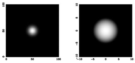
Here we are contrasting two different ways of displaying the same image. On the left is the default display of a Gaussian, whereas on this right is the result when mapping the pixels to a range from -10 to 10 with a logarithmic transfer function. Here we show the use of the ITF and and Transform options. Note that using Transform in conjunction with Pix is going to lead to unwanted results!
Colour bar/wedge
It is often desirable to annotate an image with a colour wedge showing the range of values in the image. This is accomplished with the draw_wedge function in PDL::Graphics::PGPLOT (but you can avoid calling this directly by setting the DrawWedge option in your call to imag , see above). This function should normally give a decent result without the user setting any options except the Label option which sets the annotation, but occasionally it is necessary to change its behavior and that is done by setting the following options:
Side
What side the wedge will appear on, the default is the right side and it is specified as a single character, ' B ' for bottom, ' L ', ' T ' and ' R ' for left, top and right respectively.
Displacement
The distance away from the axis. Default=2.
Width
The width of the wedge. Default=3
Foreground
The value to set the foreground colour to. This can be referred to as Fg as well. The default is the max value used by imag when drawing the image.
Background
The value to set the background colour to. This can be referred to as Bg as well. The default is the min value used by imag when drawing the image.
Label
The label used to annotate the wedge.
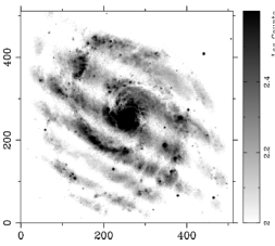
dev '/xs', {WindowWidth => 6, Aspect => 1};
$im = rfits('Frei/n4013lJ.fits');
$im += abs(min($im)-1);
$im = log10($im);
imag($im, {PlotPosition => [0.1, 0.85, 0.175, 0.925], Min => 2.6, Max
=> 2.0 });
draw_wedge({Wedge => {Width => 4, Label => 'Log Counts', Displacement
=> 1}});
Note that you will sometimes need to directly set the plot size to avoid clipping in the display. A full example that shows the use of draw_wedge can be seen in the Figure above where we display a galaxy and display a look-up table next to it.
Contour plots and vector fields
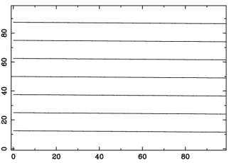
Contour plots are very similar to image displays and display lines at particular levels of the image. The function to create contour plots is cont which at the simplest level only takes a 2D array as its argument.
$a = sequence(100,100); cont $a;
That might be all you need, but most likely you would like to specify contour levels, label contours and maybe draw them in different colours.
You use the option Contours to give the wanted contour levels as a piddle and Labels to give an anonymous array of strings for labels as shown in the example below:
use PDL; use PDL::Graphics::PGPLOT;
dev('/xs');
$y = ylinvals(zeroes(100,100), -5, 5);
$x = xlinvals(zeroes(100,100), -5, 5);
$z = cos($x**2)+sin($y*2);
cont $z, {Contours => pdl(-1, 0, 1), Labels => ['-1', '0', '1']};
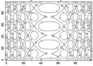
In addition it is possible to colour the labels differently from the contour lines (LabelColour), to specify the number of contours instead of their values (NContours) and to draw negative contours as dashed lines and positive as solid lines by setting the option Follow to a value >0.
Overlaying a contour plot on top of an image is as easy as displaying the image, call hold and display the contour plot. The reader might want to try a colour version of the example above ( $z as in the example):
pdl> ctab('Fire');
pdl> imag $z; hold;
pdl> cont $z, {Contours => pdl(-1,0,1)};
The final 2D plot command we will deal with here is the command for plotting a vector field, vect. This command takes two arrays as arguments. The first gives the horizontal component and the second the vertical component of the vector field. The length of the vectors can be set using the SCALE option and the position relative to the pixel centers with the option POS.
What is important to note with a command like vect is that you can use the Transform option to map a smaller vector array to a larger image. This is often useful because a vector field with 256 x 256 arrows on top of a similarly sized image will quickly be unreadable. The result of using this technique is shown below together with the code that produced the plot.
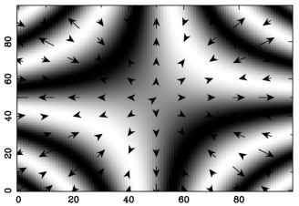
pdl> $x = xlinvals(zeroes(100,100), -5, 5)
pdl> $y = ylinvals(zeroes(100,100), -5, 5)
pdl> $z = sin($x*$y/2)
pdl> imag $z;
pdl> hold;
# Show the partial derivatives wrt. x & y as vectors
pdl> $xcomp = $x*cos($x*$y/2)/2
pdl> $ycomp = $y*cos($x*$y/2)/2
# We want to show only every tenth vector for clarity
pdl> $s = '0:-1:10,0:-1:10';
# Finally we need to map the final 10x10 array to the 100x100 image
pdl> $tr = pdl(0,10,0,0,0,10)
pdl> vect $xcomp->slice($s), $ycomp->slice($s), {Transform=>$tr}
Drawing simple shapes
In addition to the simple commands described above, there are a few convenient commands for drawing simple shapes such as circles, ellipses and rectangles. These are fairly straightforward commands with similar options and invocations so we will go through them fairly quickly. A common issue with these commands as with the poly command is that they draw filled shapes, if you want outlined shapes to be drawn you have to set the Filltype option to Outline.
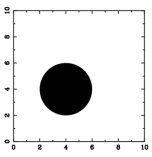
The circle command is probably the simplest, it draws a circle (which may or may not look like a circle depending on the aspect ratio of your display - see Setting up the plot area. The user specifies the radius and the x and y position of the center:
pdl> dev '/xs', {Aspect => 1, WindowWidth => 5}
pdl> env 0, 10, 0, 10
pdl> $radius=2; ($x, $y) = (4, 4)
pdl> circle $x, $y, $radius, {LineWidth => 3}
The ellipse function is like the circle function but it requires the user to specify the minor and major axis and the angle between the major axis and the horizontal. For ease of use it is probably better to specify these as options, but if you remember the order you can also give them directly as arguments to the function (x-position, y-position, major axis, minor axis, angle):
pdl> dev '/xs', {Aspect => 1, WindowWidth => 5}
pdl> env 0, 10, 0, 10
pdl> ellipse 4, 4, {MajorAxis => 2, MinorAxis => 1, Theta =>
atan2(1,1)}