Radio Frequency by Steve Winder and Joe Carr - HTML preview

1.4 Formation of radio waves

Radio waves are electromagnetic. They contain both electric and magnetic fields at right angles to each other and also at right angles to the direction of propagation. An alternating current flowing in a conductor produces an alternating magnetic field surrounding it and an alternating voltage gradient – an electric field – along the length of the conductor. The fields combine to radiate from the conductor as in Figure 1.3.

E plane
^E H plane_I
H field
Figure 1.3 Formation of electromagnetic wave

The plane of the electric field is referred to as the E plane and that of the magnetic field as the H plane. The two fields are equivalent to the voltage and current in a wired circuit. They are measured in similar terms, volts per metre and amperes per metre, and the medium through which they propagate possesses an impedance. Where E = ZI in a wired circuit, for an electromagnetic wave:

E = ZH

where
E = the RMS value of the electric field strength, V/metre H = the RMS value of the magnetic field strength, A/metre Z = characteristic impedance of the medium, ohms

The voltage is that which the wave, passing at the speed of light, would induce in a conductor one metre long.

The characteristic impedance of the medium depends on its permeability (equivalent of inductance) and permittivity (equivalent of capacitance). Taking the accepted figures for free space as:

µ = 4π × 10⁻⁷ henrys (H) per metre (permeability) and ε = 1/36π × 10⁹ farads (F) per metre (permittivity)

 

then the impedance of free space, Z, is given by:

 

^µ 120π = 377 ohms_ε =

The relationship between power, voltage and impedance is also the same for electromagnetic waves as for electrical circuits, W = E²/Z. The simplest practical radiator is the elementary doublet formed by opening out the ends of a pair of wires. For theoretical considerations the length of the radiating portions of the wires is made very short in relation to the wavelength of the applied current to ensure uniform current distribution throughout their length. For practical applications the length of the radiating elements is one half-wavelength (λ/2) and the doublet then becomes a dipole antenna (Figure 1.4).

When radiation occurs from a doublet the wave is polarized. The electric field lies along the length of the radiator (the E plane) and the magnetic field (the H plane) at right angles to it. If the E plane is vertical, the radiated field is said to vertically polarized. Reference to the E and H planes avoids confusion when discussing the polarization of an antenna.

Unlike the isotropic radiator, the dipole possesses directivity, concentrating the energy in the H plane at the expense of the E plane. It effectively provides a power gain in the direction of the H plane

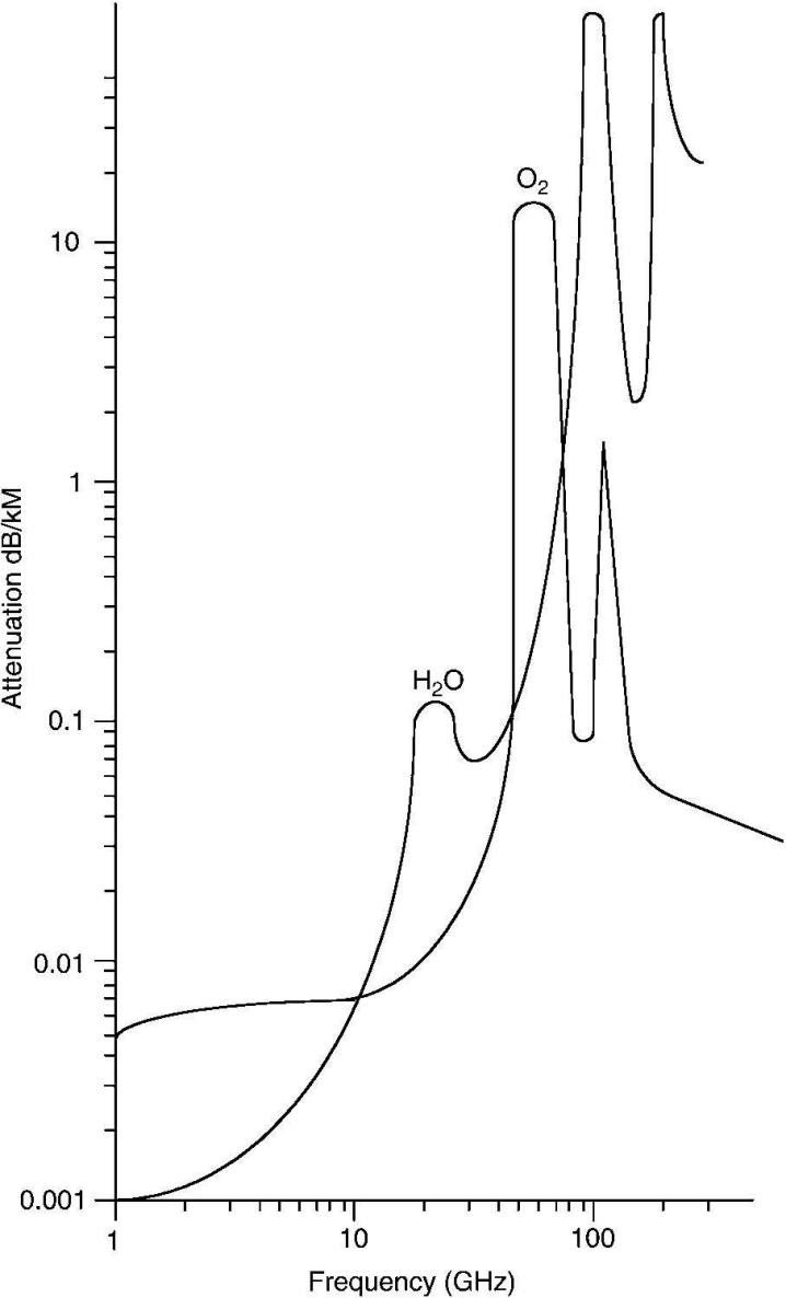
From^l transmitter²
Voltage distribution Current distribution Figure 1.4 Doublet (dipole) antenna
180
170 7000 MHz
3500 MHz ¹⁶⁰ 2000 MHz 1000 MHz 150
400 MHz ¹⁴⁰ 200 MHz
₁₃₀ 100 MHz
120
110

100 Figure 1.6 Major loss of microwave communications and radar systems due to atmospheric attenuation

90
10 20 30 50 70 100 200 300 500 700 1000 Distance (km)
Figure 1.5 Free space loss vs. distance and frequency

 

 

compared with an isotropic radiator. This gain is 1.6 times or 2.15 dBi (dBi means dB relative to an isotropic radiator).

For a direct ray the power transfer between transmitting and receiving isotropic radiators is inversely proportional to the distance between them in wavelengths. The free space power loss is given by:

Free space loss, dB

 

=

 

10 log

 

(4πd)²

 

10_λ2

 

where d and λ are in metres, or:

 

Free space loss (dB) = 32.4+ 20× log₁₀d + 20× log₁₀ f

 

where d = distance in km and f = frequency in MHz.

The free space power loss, therefore, increases as the square of the distance and the frequency. Examples are shown in Figure 1.5.
With practical antennas, the power gains of the transmitting and receiving antennas, in dBi, must be subtracted from the free space loss calculated as above. Alternatively, the loss may be calculated by:

(4πd)² 1 Free space loss (dB) = 10 log_{10 λ2} ×_{Gt × Gr}

 

where G_t and G_r are the respective actual gains, not in dB, of the transmitting and receiving antennas.

A major loss in microwave communications and radar systems is atmospheric attenuation (see Figure 1.6). The attenuation (in decibels per kilometre (dB/km)) is a function of frequency, with especial problems showing up at 22 GHz and 64 GHz. These spikes are caused by water vapour and atmospheric oxygen absorption of microwave energy, respectively. Operation of any microwave frequency requires consideration of atmospheric losses, but operation near the two principal spike frequencies poses special problems. At 22 GHz, for example, an additional 1 dB/km of loss must be calculated for the system.