Radio frequency transmission lines possess similar electrical characteristics to base band lines. However, they may be carrying large powers and the effects of a mismatched load are much more serious than a loss of transferred power. Three types of wire RF line are commonly used: a single wire with ground return for MF and LF broadcast transmission, an open pair of wires at HF and co-axial cable at higher frequencies. Waveguides are used at the higher microwave frequencies. RF lines exhibit an impedance characterized by their type and construction.
The physical dimensions of an RF transmission line, the spacing between the conductors, their diameters and the dielectric material between them, determine the characteristic impedance of the line, Z0, which is calculated for the most commonly used types as follows.
Single wire with ground return (Figure 3.3(a)):4h Z0 = 138 log10 d ohms
2-wire balanced, in air (Figure 3.3(b)):
Z
0
=
276log 2s
10 d ohms√εp
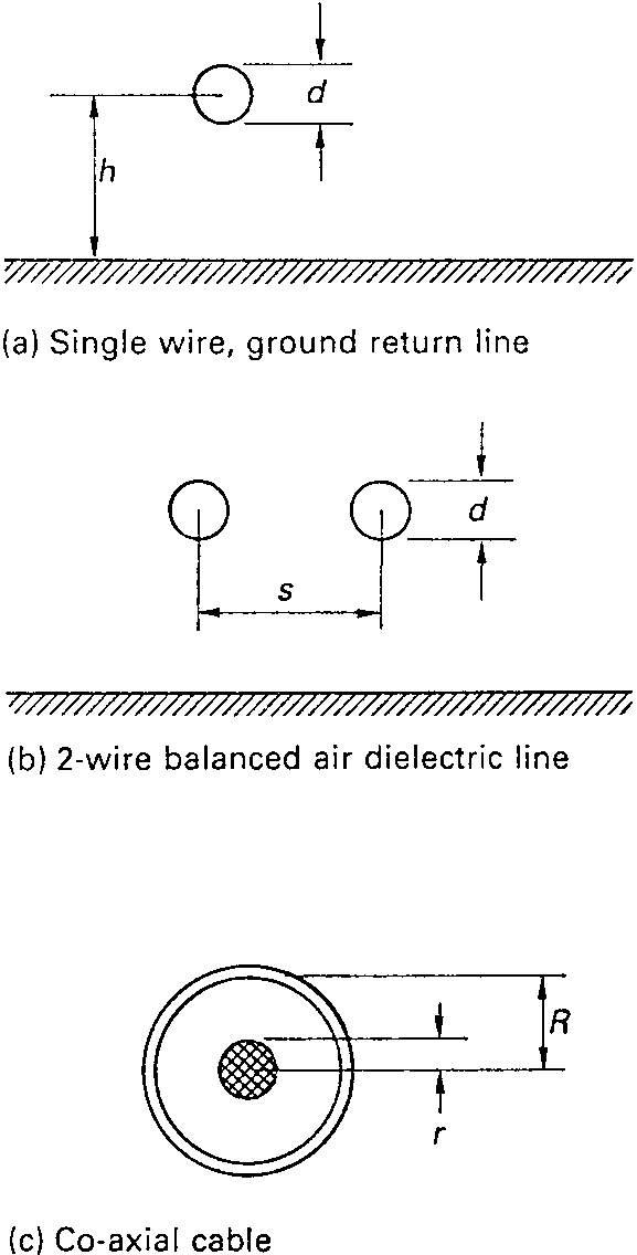 Figure 3.3
Co-axial (Figure 3.3(c)):
Z
0
=
138log R
10 r ohms√εr
where dimensions are in mm and εr = relative permittivity of continuous dielectric.
The loss in RF cables is quoted in specifications as attenuation in dB per unit length at specific frequencies, the attenuation increasing with frequency. The electrical specifications for cables having a braided outer conductor are given in Tables 3.1 and 3.2. Those for the now commonly used foam dielectric, solid outer conductor cables are provided in Table 3.3.
Table 3.1 RF cables USA RG and URM seriesAttenuation (dB per 100 ft)
RG-6A/U 75.0 0.332
Velocity0.659 0.21 0.78 2.9
RG-11A/U 75.0 0.405 0.66 0.18 0.7 2.3
RG-12A/U 75.0 0.475 0.659 0.18 0.66 2.3
RG-16/U 52.0 0.630 0.670 0.1 0.4 1.2
RG-34A/U 75.0 0.630 0.659 0.065 0.29 1.3
RG-34B/U 75.0 0.630 0.66 – 0.3 1.4
RG-35A/U 75.0 0.945 0.659 0.07 0.235 0.85 RG-54A/U 58.0 0.250 0.659 0.18 0.74 3.1
RG-55/U 53.5 0.206 0.659 0.36 1.3 4.8
RG-55A/U 50.0 0.216 0.659 0.36 1.3 4.8
RG-58/U 53.5 0.195 0.659 0.33 1.25 4.65 11.2 21.0
Capacity20.0
voltage2700 7.8 16.5 20.5 5000 8.0 16.5 20.5 4000 6.7 16.0 29.5 6000 6.0 12.5 20.5 5200 5.8 – 21.5 6500 3.5 8.60 20.5 10 000 11.5 21.5 26.5 3000 17.0 32.0 28.5 1900 17.0 32.0 29.5 1900 17.5 37.5 28.5 1900 (continued overleaf) Table 3.1 (continued)
RG-58C/U 50.0 RG-59A/U 75.0 RG-59B/U 75 RG-62A/U 93.0 RG-83/U 35.0 RG-174A/U 50 RG-188A/U 50
∗ RG-213/U 50
†RG-218/U 50
‡RG-220/U 50
URM43 50
URM70 75
URM76 50
0.195
Velocity0.659 0.42 1.4 4.9
0.242 0.659 0.34 1.10 3.40
0.242 0.66 – 1.1 3.4
0.242 0.84 0.25 0.85 2.70
0.405 0.66 0.23 0.80 2.8
0.1 0.66 1.83 3.35 11.0
0.11 0.66 – – 10.0
0.405 0.66 0.16 0.6 1.9
0.870 0.66 0.066 0.2 1.0
1.120 0.66 0.04 0.2 0.7
0.116 0.66 0.396 1.25 3.96
0.128 0.66 0.457 1.46 4.63
0.116 0.66 0.457 1.46 4.72 24.0 45.0
Capacity30.0
voltage1900 12.0 26.0 20.5 2300 12.0 – 21 2300 8.6 18.5 13.5 750 9.6 24.0 44.0 2000 32.0 64.0 30.0 1400 30.0 – – 1200 8.0 – 29.5 5000 4.4 – 29.5 11 000 3.6 – 29.5 14 000 – – 30.0 2600 – – 20.5 1800 – – 30.0 2600 Table 3.2 British UR series
∗ Formerly RG8A/U. †Formerly RG17A/U. ‡Formerly RG19A/U.
Attenuation (dB per 100 ft)43
number Nominal52 0.195 (inches)0.032 Capacity29 voltage2750 1.3 4.3 8.7 18.1 Nearest equivalent58/U
57 75 0.405 0.044 20.6 5000 0.6 1.9 3.5 7.1 11A/U
63∗ 75 0.855 0.175 14 4400 0.15 0.5 0.9 1.7
67 50 0.405 7/0.029 30 4800 0.6 2.0 3.7 7.5 213/U
74 51 0.870 0.188 30.7 15 000 0.3 1.0 1.9 4.2 218/U
76 51 0.195 19/0.0066 29 1800 1.6 5.3 9.6 22.0 58C/U
77 75 0.870 0.104 20.5 1 25 000 0.3 1.0 1.9 4.2 164/U
79∗ 50 0.855 0.265 21 6000 0.16 0.5 0.9 1.8
83∗ 50 0.555 0.168 21 2600 0.25 0.8 1.5 2.8
85∗ 75 0.555 0.109 14 2600 0.2 0.7 1.3 2.5
90 75 0.242 0.022 20 2500 1.1 3.5 6.3 12.3 59B/U Table 3.3 Foam dielectric, solid outer conductor co-axial RF cables 50 ohms characteristic impedance
Cable type FSJ1-50A FSJ4-50B LDF2-50 LDF4-50A 1/4 1/2 3/8 1/2
Min. bending 1.0 1.25 3.75 5.0
radius, in. (mm) (25) (32) (95) (125)
Propagation 84 81 88 88
velocity, %
Max. operating 20.4 10.2 13.5 8.8
frequency, GHz
Att. dB/100 ft
(dB/100 m)
50 MHz 1.27 0.732 0.75 0.479 (4.17) (2.40) (2.46) (1.57)
100 MHz 1.81 1.05 1.05 0.684 (5.94) (3.44) (3.44) (2.24)
400 MHz 3.70 2.18 2.16 1.42 (12.1) (7.14) (7.09) (4.66)
1000 MHz 6.00 3.58 3.50 2.34 (19.7) (11.7) (11.5) (7.68)
5000 MHz 14.6 9.13 8.80 5.93 (47.9) (30.0) (28.9) (19.5)
10 000 MHz 21.8 15.0 13.5 N/A (71.5) (49.3) (44.3) N/A
Power rating, kW
at 25æC(77æF)
50 MHz 1.33 3.92 2.16 3.63
100 MHz 0.93 2.74 1.48 2.53
400 MHz 0.452 1.32 0.731 1.22
1000 MHz 0.276 0.796 0.445 0.744
5000 MHz 0.11 0.30 0.17 0.29
10 000 MHz 0.072 0.19 0.12 N/A
1. Lower attenuation
2. Improved RF shielding, approximately 30 dB improvement
3. High average power ratings because of the improved thermal conductivity of the outer conductor and the lower attenuation.
When an RF cable is mismatched, i.e. connected to a load of a different impedance to that of the cable, not all the power supplied to the cable is absorbed by the load. That which does not enter the load is reflected back down the cable. This reflected power adds to the incident voltage when they are in phase with each other and subtracts from the incident voltage when the two are out of phase. The result is a series of voltage – and current – maxima and minima at halfwavelength intervals along the length of the line (Figure 3.4). The maxima are referred to as antinodes and the minima as nodes.
Incident current phaseThe voltage standing wave ratio is the numerical ratio of the maximum voltage on the line to the minimum voltage: VSWR = Vmax/Vmin. It is also given by: VSWR = RL/Z0 or Z0/RL (depending on which is the larger so that the ratio is always greater than unity) where RL = the load resistance.
The return loss is the power ratio, in dB, between the incident (forward) power and the reflected (reverse) power.
The reflection coefficient is the numerical ratio of the reflected voltage to the incident voltage.
The VSWR is 1, and there is no reflected power, whenever the load is purely resistive and its value equals the characteristic impedance of the line. When the load resistance does not equal the line impedance, or the load is reactive, the VSWR rises above unity.
A low VSWR is vital to avoid loss of radiated power, heating of the line due to high power loss, breakdown of the line caused by high voltage stress, and excessive radiation from the line. In practice, a VSWR of 1.5:1 is considered acceptable for an antenna system, higher ratios indicating a possible defect.
Use can be made of standing waves on sections of line to provide filters and RF transformers. When a line one-quarter wavelength long (aλ/4 stub) is open circuit at the load end, i.e. high impedance, an effective short-circuit is presented to the source at the resonant frequency of the section of line, producing an effective band stop filter. The same effect would be produced by a short-circuited λ/2 section. Unbalanced co-axial cables with an impedance of 50 are commonly used to connect VHF and UHF base stations to their antennas although the antennas are often of a different impedance and balanced about ground. To match the antenna to the feeder and to provide a balance to unbalance transformation (known as a balun), sections of co-axial cable are built into the antenna support boom to act as both a balun and an RF transformer.
The sleeve balun consists of an outer conducting sleeve, one quarterwavelength long at the operating frequency of the antenna, and connected to the outer conductor of the co-axial cable as in Figure 3.5. When viewed from point Y, the outer conductor of the feeder cable and the sleeve form a short-circuited quarter-wavelength stub at the operating frequency and the impedance between the two is very high. This effectively removes the connection to ground for RF, but not for DC, of the outer conductor of the feeder cable permitting the connection of the balanced antenna to the unbalanced cable without short-circuiting one element of the antenna to ground.
Balanced Concentric sleeve dipoleCo-axial cable Y l
4
If a transmission line is mismatched to the load variations of voltage and current, and therefore impedance, occur along its length (standing waves). If the line is of the correct length an inversion of the load impedance appears at the input end. When a λ/4 line is terminated in other than its characteristic impedance an impedance transformation takes place. The impedance at the source is given by:
Zs
=
Z02 ZL
where
Zs = impedance at input to line
Z0 = characteristic impedance of line
ZL = impedance of load
By inserting a quarter-wavelength section of cable having the correct characteristic impedance in a transmission line an antenna of any impedance can be matched to a standard feeder cable for a particular design frequency. A common example is the matching of a folded dipole of 300 impedance to a 50 feeder cable.
Let Zs = Z0 of feeder cable and Z0 = characteristic impedance of transformer section. Then:Z
0
=
Z0 ZL
2
Z0 = Z0ZL
= √300× 50 = 122