1 0 1 0 1 0
(73)
x
2
x 3
x 4
and
1
T 0
(74)
x
1
142
Applications of Nonlinear Control
From this we see that the function 1
T should be a function of x 1 alone. Therefore, we take
the simplest solution
y
1
1
T
x 1
(75)
and compute
y
2
2
T
d 1
T , f
x 2
(76)
MgL
k
y
3
3
T
d 2
T , f
sin( x 1)
( x 1 x 3)
(77)
I
I
MgL
k
y
4
4
T
d 3
T , f
cos( x 1) x 2
( x 2 x 4)
(78)
I
I
The feedback linearizing control input u is found from the condition
1
u
( v d
4
T , f )
dT , g
4
(79)
IJ
( v (
a x)) ( x) v ( x)
k
where
MgL
MgL
k
k
k k MgL
2
( x) :
sin( x
1 )( x 2
cos( x 1)
)
( x 1 x 3)(
cos( x 1)) (80)
I
I
I
I
I
J
I
Therefore in the coordinates y 1,, y 4 with the control law (79) the system becomes
y
1
y 2 y 2 y 3
y
3
y 4 y 4 v
or, in matrix form,
y Ay bv
(81)
where
0 1 0 0
0
0 0 1 0
0
A
b
0 0 0 1
0
0 0 0 0
1
The transformed variables y 1,, y 4 are themselves physically meaningful. We see that
y
1
x 1 =link position
Predictive Function Control of the Single-Link Manipulator with Flexible Joint
143
y
2
x 2 =link velocity
y
3
y 2 =link acceleration
y
4
y 3 =link jerk
Since the motion trajectory of the link is typically specified in terms of these quantities they
are natural variables to use for feedback.
For given a linear system in state space form, such as (81), a state feedback control law is an
input v of the form
4
T
v k y r k
iyi
r
(82)
i1
where ki are constants and r is a reference input. If we substitute the control law (82) into
(81), we obtain
(
T
y
A bk ) y br
(83)
Thus we see that the linear feedback control has the effect of changing the poles of the
system from those determined by A to those determined by
T
A bk
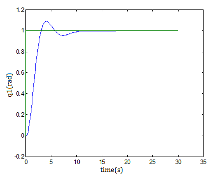
When the parameters are chosen k
1
62.5 , k
2
213.6 , k
3
204.2 k
4
54 , we can get step
responses in Figure 4. where k1, k2, k3 and k4 are linear feedback coefficients to place the
eigenvalues of A in a desired location.
y1 0
1
0
0 y 1 0
y
0
0
1
0 y 0
2
2
r
(84)
y
3
0
0
0
1
y 3
0
y
4 62.5
213.8
204.2
54 y 4 1
y 1
y
y 1 0 0 0 2
(85)
y
3
y 4
The internal model parameter: K 0.016
M
,
3
M
T , 8
d , and the coincidence point H=10.
Response time of reference trajectory is 0.01, and sample time is 0.01.
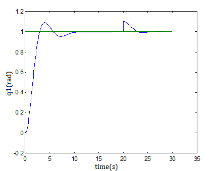
For the uncertainty , the system (38) can be written in matrix form as
(
T
y
A bk ) y {
b r ( y, v)}
then use predictive function control strategy to reduce or overcome uncertainty of nonlinear
feedback error ( y, v) ,and simulation result is shown in Figure 5 for ( y, v) 10% yr .
144
Applications of Nonlinear Control
Fig. 4. link position output
Predictive Function Control of the Single-Link Manipulator with Flexible Joint
145
Fig. 5. link position output with uncertainty rejection
146
Applications of Nonlinear Control
6. Conclusion
A new three stage design method is presented for the single link manipulator with flexible
joint. The first is feedback linearization; the second is to use pole placement to satisfy
performance, and the third is to develop predictive function control to compensate
uncertainty. Finally, for the same uncertainty, robustness is better than traditional method.
7. References
Khorasani, K. (1990). Nonlinear feedback control of flexible joint manipulators: a single link
case study. IEEE Transactions on Automatic Control, Vol. 35, No. 10, pp. 1145-1149,
ISSN 0018-9286
Richalet, J.; Rault, A.; Testud, J. L.; Papon, J.(1978). Model predictive heuristic control:
Applications to industrial processes. Automatica, Vol. 14, No. 5, pp. 413-428, ISSN
0005-1098
Spong, M.W.; Khorasani, K. & Kokotovic P.V. (1987). An integral manifold approach to the
feedback control of flexible joint robots. IEEE Journal of Robotics and Automation, Vol.
RA-3, No. 4, pp. 291-300, ISSN 0882-4967
Spong, M.W.(1987). Modeling and control of elastic joint robots. Journal of Dyn. Sys. Meas.
and Cont. , Vol. 109, pp.310-319, ISSN 0022-0434
Spong, M.W. (1989). On the force control problem for flexible joint manipulator. IEEE
Transactions on Automatic Control, Vol. 34, No. 1, pp. 107-111, ISSN 0018-9286
E. F. Camacho, Carlos Bordons(2004). Model predictive control. Springer-Verlag London Berlin
Limited. ISBN 1-85233-694-3
9
On Optimization Techniques for a Class
of Hybrid Mechanical Systems
Vadim Azhmyakov and Arturo Enrique Gil García
Department of Control Automation, CINVESTAV, A.P. 14-740, Mexico D.F.,
Mexico
1. Introduction
Several classes of general hybrid and switched dynamic systems have been extensively
studied, both in theory and practice [3,4,7,11,14,17,19,26,27,30].
In particular, driven by
engineering requirements, there has been increasing interest in optimal design for hybrid
control systems [3,4,7,8,13,17,23,26,27]. In this paper, we investigate some specific types of
hybrid systems, namely hybrid systems of mechanical nature, and study the corresponding
hybrid OCPs. The class of dynamic models to be discussed in this work concerns hybrid
systems where discrete transitions are being triggered by the continuous dynamics. The
control objective (control design) is to minimize a cost functional, where the control
parameters are the conventional control inputs.
Recently, there has been considerable effort to develop theoretical and computational
frameworks for complex control problems. Of particular importance is the ability to operate
such systems in an optimal manner. In many real-world applications a controlled mechanical
system presents the main modeling framework and can be specified as a strongly nonlinear
dynamic system of high order [9,10,22]. Moreover, the majority of applied OCPs governed
by sophisticated real-world mechanical systems are optimization problems of the hybrid
nature. The most real-world mechanical control problems are becoming too complex to allow
analytical solution. Thus, computational algorithms are inevitable in solving these problems.
There is a number of results scattered in the literature on numerical methods for optimal
control problems. One can find a fairly complete review in [3,4,8,24,25,29]. The main idea
of our investigations is to use the variational structure of the solution to the specific two point
boundary-value problem for the controllable hybrid-type mechanical systems in the form of
Euler-Lagrange or Hamilton equation and to propose a new computational algorithm for the
associated OCP. We consider an OCP in mechanics in a general setting and reduce the initial
problem to a constrained multiobjective programming. This auxiliary optimization approach
provides a basis for a possible numerical treatment of the original problem.
The outline of our paper is as follows.
Section 2 contains some necessary basic facts
related to the conventional and hybrid mechanical models.
In Section 3 we formulate
and study our main optimization problem for hybrid mechanical systems. Section 4 deals
with the variational analysis of the OCP under consideration. We also briefly discuss the
148
2
Will-be-set-by-IN-TECH
Applications of Nonlinear Control
computational aspect of the proposed approach. In Section 5 we study a numerical example
that constitutes an implementable hybrid mechanical system. Section 6 summarizes our
contribution.
2. Preliminaries and some basic facts
Let us consider the following variational problem for a hybrid mechanical system that is
characterized by a family of Lagrange functions { ˜ Lp }, p
i
i ∈ P
1 r
minimize
∑ β[
(
t
t, q( t), ˙ q( t)) dt
0
i− 1, ti ) ( t) ˜
Lpi
i=1
(1)
subject to q(0) = c 0, q(1) = c 1,
where P is a finite set of indices (locations) and q( ·) ( q( t) ∈ R n) is a continuously differentiable function. Here β[ ti− 1, ti)( ·) are characteristic functions of the time intervals [ ti− 1, ti), i = 1, ..., r associated with locations. Note that a full time interval [0, 1] is assumed to be separated into
disjunct sub-intervals of the above type for a sequence of switching times:
τ := {t 0 = 0, t 1, ..., tr = 1 }.
We refer to [3,4,7,8,13,17,23,26,27] for some concrete examples of hybrid systems with the
above dynamic structure.
Consider a class of hybrid mechanical systems that can be
represented by n generalized configuration coordinates q 1, ..., qn. The components ˙ qλ( t), λ =
1, ..., n of ˙ q( t) are the so-called generalized velocities. Moreover, we assume that ˜ Lp ( t, ·, ·) i
are twice continuously differentiable convex functions. It is well known that the formal
necessary optimality conditions for the given variational problem (1) describe the dynamics of
the mechanical system under consideration. This description can be given for every particular
location and finally, for the complete hybrid system. In this contribution, we study the hybrid
dynamic models that free from the possible external influences (uncertainties) or forces. The
optimality conditions for mentioned above can be rewritten in the form of the second-order
Euler-Lagrange equations (see [1])
d ∂ ˜ Lp ( t, q, ˙ q)
∂ ˜ L ( t, q, ˙ q)
i
−
pi
= 0, λ = 1, ..., n ,
dt
∂ ˙ qλ
∂qλ
(2)
q(0) = c 0, q(1) = c 1,
for all pi ∈ P. The celebrated Hamilton Principle (see e.g., [1]) gives an equivalent variational
characterization of the solution to the two-point boundary-value problem (2).
For the controllable hybrid mechanical systems with the parametrized (control inputs)
Lagrangians Lp ( t, q, ˙ q, u), p
i
i ∈ P we also can introduce the corresponding equations of
motion
d ∂Lp ( t, q, ˙ q, u)
∂L ( t, q, ˙ q, u)
i
−
pi
= 0,
dt
∂ ˙ qλ
∂qλ
(3)
q(0) = c 0, q(1) = c 1,
On Optimization Techniques for a Class of Hybrid Mechanical Systems
149
On Optimization Techniques for a Class of Hybrid Mechanical Systems
3
where u( ·) ∈ U is a control function from the set of admissible controls U . Let
U := {u ∈ R m : b 1, ν ≤ uν ≤ b 2, ν, ν = 1, ..., m},
U := {v( ·) ∈ L2 m([0, 1]) : v( t) ∈ U a.e. on [0, 1] }, where b 1, ν, b 2, ν, ν = 1, ..., m are constants. The introduced set U provides a standard example of an admissible control set. In this specific case we deal with the following set of admissible
controls U
C1 m(0, 1). Note that Lp depends directly on the control function u( ·). Let us
i
assume that functions Lp ( t, ·, ·, u) are twice continuously differentiable functions and every i
Lp ( t, q, ˙ q, ·) is a continuously differentiable function. For a fixed admissible control u( ·) we i
obtain for all pi ∈ P the above hybrid mechanical system with ˜ Lp ( t, q, ˙ q) ≡ L ( t, q, ˙ q, u( t)).
i
pi
It is also assumed that Lp ( t, q, ·, u) are strongly convex functions, i.e., for any
i
( t, q, ˙ q, u) ∈ R × R n × R n × R m, ξ ∈ R n the following inequality
n
n
∑ ∂ 2 Lp ( t, q, ˙ q, u)
i
ξλξθ ≥ α ∑ ξ 2 λ, α > 0
λ