i
i tj+1 := ti
i
consider the corresponding finite-dimensional optimization problem
minimize JN ( qN( ·), uN( ·)) and PN( qN( ·)),
( qN( ·), uN( ·)) ∈ (
Γ N) × ( U N
C 1 (
i
m, N 0, 1)),
(10)
i=1,..., r
where JN and PN are discrete variants of the objective functionals J and P from (7). Moreover,
Γ N is a correspondingly discrete set Γ
(0, 1) is set of suitable discrete functions
i
i and C 1
m, N
that approximate the trajectories set C 1 m(0, 1). Note that the initial continuous optimization
problem can also be presented in a similar discrete manner. For example, we can introduce
the (Euclidean) spaces of piecewise constant trajectories qN ( ·) and piecewise constant control
functions uN ( ·). As we can see the Banach space C1 n(0, 1) and the Hilbert space L2 m([0, 1]) will be replaced in that case by some appropriate finite-dimensional spaces.
The discrete optimization problem (10) approximates the infinite-dimensional optimization
problem (7). We assume that the set of all weak Pareto optimal solution of the discrete
problem (10) is nonempty. Moreover, similarly to the initial optimization problem (7) we
also assume that the discrete problem (10) is regular. If P( ·) is a convex functional, then the
discrete multiobjective optimization problem (10) is also a convex problem. Analogously to
the continuous case (7) or (8) we also can write the corresponding KKT optimality conditions
for a finite-dimensional optimization problem over the set of variables ( qN( ·), uN( ·)). The
necessary optimality conditions for a discretized problem (10) reduce the finite-dimensional
multiobjective optimization problem to a system of nonlinear equations. This problem can be
solved by some gradient-based or Newton-type methods (see e.g., [24]).
Finally, note that the proposed numerical approach uses the necessary optimality conditions,
namely the KKT conditions, for the discrete variant (10) of the initial optimization problem (7).
It is common knowledge that some necessary conditions of optimality for discrete systems, for
example the discrete version of the classical Pontryagin Maximum Principle, are non-correct
in the absence of some restrictive assumptions. For a constructive numerical treatment of
the discrete optimization problem it is necessary to apply some suitable modifications of
the conventional optimality conditions. For instance, in the case of discrete optimal control
problems one can use so-called Approximate Maximum Principle which is specially designed
for discrete approximations of general OCPs [21].
5. Mechanical example
This section is devoted to a short numerical illustration of the proposed hybrid approach
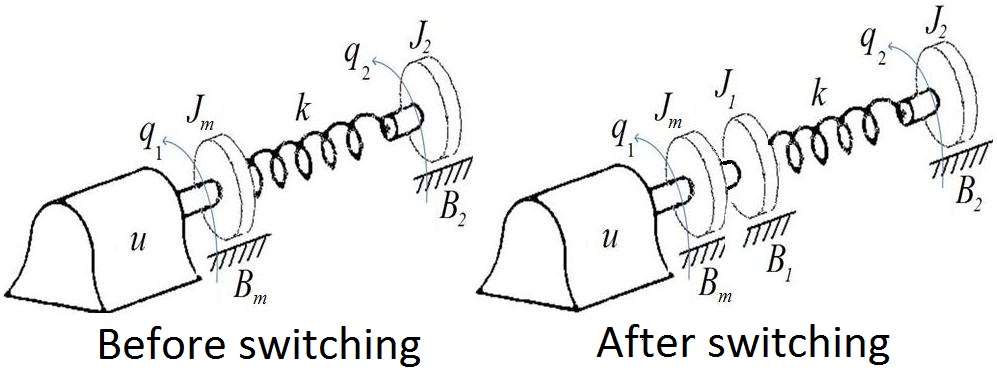
to mechanical systems. We deal with a practically motivated model that has the following
structure (see Fig. 1).
Let us firstly describe the parameters of the mechanical model under consideration:
On Optimization Techniques for a Class of Hybrid Mechanical Systems
157
On Optimization Techniques for a Class of Hybrid Mechanical Systems
11
Fig. 1. Mechanical example
• q 1 it corresponds to the position of motor.
• q 2 is the position of inertia J 2.
• J 1, J 2 are the external inertias.
• Jm is an inertia of motor.
• Bm it corresponds to the friction of the motor.
• B 1, B 2 they correspond to the frictions of the inertias J 1, J 2.
• k is a constant called the rate or spring constant.
• u it corresponds to the torque of motor.
The relations for the kinetic potential energies give a rise to the corresponding Lagrange
dynamics:
K( t) = 1 J
+ 1 J
2 m ˙ q 21
2 2 ˙ q 22
V( t) = 1 k ( q
2
1 − q 2)2
Finally, we have
L( q( t), ˙ q( t)) = 1 J
+ 1 J
− 1 k ( q
2 m ˙ q 21
2 2 ˙ q 22
2
1 − q 2)2
and the Euler-Lagrange equation with respect to the generalized coordinate q 1 has the
following form
Jm ¨ q 1 + Bm ˙ q 1 − k( q 2( t) − q 1( t)) = u( t) (11)
We now considered the Euler-Lagrange equation with respect to the second generalized
variable, namely, with respect to q 2
d ∂L( q( t), ˙ q( t)) − ∂L( q( t), ˙ q( t)) = −B
dt
∂ ˙ q
2 ˙
q 2( t)
2
∂q 2
We get the next relation
J 2 ¨ q 2( t) + B 2 ˙ q 2( t) + k( q 2( t) − q 1( t)) = 0
158
12
Will-be-set-by-IN-TECH
Applications of Nonlinear Control
The redefinition of the states x 1 := q 1, x 2 := ˙ q 1, x 3 := q 2, x 4 := ˙ q 2 with X := ( x 1, x 2, x 3, x 4) T
implies the compact state-space form of the resulting equation:
⎡ ⎤
⎡
⎤ ⎡ ⎤ ⎡ ⎤
⎡ ⎤
˙ x
0
1
0
0
1
x 1
0
x 0
⎢ ⎥
⎢ −
1
k −Bm
k
0 ⎥ ⎢
⎥ ⎢ 1 ⎥
⎢ ⎥
˙
˙ x
⎢
⎥ x
x 0
X := ⎢ 2
J
J
J
2
⎣ ⎥
⎢ m
m
m
⎥ ⎢ ⎥ ⎢ Jm ⎥
⎢ 2⎥
˙ x ⎦ =
⎣ ⎦ + ⎣ ⎦ u, X 0 := ⎣ ⎦
(12)
3
⎣ 0
0
0
1 ⎦ x 3
0
x 03
˙ x
k
−B
4
0
−k
2
x
0
x 0
J
4
2
J 2
J 2
4
The switching structure of the system under consideration is characterized by an additional
inertia J 1 and the associated friction B 1. The modified energies are given by the expressions:
the kinetic energy:
K( t) = 1 J
+ 1 J
+ 1 J
2 m ˙ q 21
2 1 ˙ q 21
2 2 ˙ q 22
the potential energy:
V( t) = 1 k ( q
2
1 − q 2)2
The function of Lagrange can be evaluated as follows
L( q, ˙ q) = 1 J
+ 1 J
+ 1 J
− 1 k ( q
2 m ˙ q 21
2 1 ˙ q 21
2 2 ˙ q 22
2
1 − q 2)2
(13)
The resulting Euler-Lagrange equations (with respect to q 1 and to q 2 can be rewritten as
( Jm + J 1) ¨ q 1( t) + ( Bm + B 1) ˙ q 1( t) − k( q 2( t) − q 1( t)) = u( t) (14)
J 2 ¨ q 2( t) + B 2 ˙ q 2( t) + k( q 2( t) − q 1( t)) = 0
Using the notation introduced above, we obtain the final state-space representation of the
hybrid dynamics associated with the given mechanical model:
⎡ ⎤
⎡
⎤ ⎡ ⎤ ⎡
⎤
˙ x
0
1
0
0
1
x 1
0
⎢ ⎥
⎢ −k −( Bm+ B 1)
k
⎥ ⎢ ⎥ ⎢ 1 ⎥
˙
˙ x
⎢
0 ⎥ x
X := ⎢ 2
2
⎣ ⎥
⎢ Jm+ J 1
Jm+ J 1
Jm+ J 1
⎥ ⎢ ⎥ ⎢ Jm+ J 1 ⎥
˙ x ⎦ =
⎣ ⎦ + ⎣
⎦ u
(15)
3
⎣ 0
0
0
1 ⎦ x 3
0
˙ x
k
−B
4
0
−k
2
x
0
J
4
2
J 2
J 2
The considered mechanical system has a switched nature with a state-dependent switching
signal. We put x 4 = − 10 for the switching-level related to the additional inertia in the system
(see above).
Our aim is to find an admissible control law that minimize the value of the quadratic costs
functional
t f
I( u( ·)) = 1
XT( t) QX( t) + uT( t) Ru( t) dt −→ min
(16)
2 t 0
u( ·)
The resulting Linear Quadratic Regulator that has the follow form
uopt( t) = −R− 1( t) BT( t) P( t) Xopt( t)
(17)
On Optimization Techniques for a Class of Hybrid Mechanical Systems
159
On Optimization Techniques for a Class of Hybrid Mechanical Systems
13
where P( t) is a solution of the Riccati equation (see [7] for details)
˙
P( t) = −( AT( t) P( t) + P( t) A( t)) + P( t) B( t) R− 1( t) BT( t) P( t) − Q( t) (18)
with the final condition
P( t f ) = 0
(19)
Let us now present a conceptual algorithm for a concrete computation of the optimal pair
( uopt, Xopt( ·)) in this mechanical example. We refer to [7, 8] for the necessary facts and the
general mathematical tool related to the hybrid LQ-techniques.
Algorithm 1. The conceptual algorithm used:
(0) Select a tswi ∈ 0, t f , put an index j = 0
(1) Solve the Riccati euqation (18) for (15) on the time intervals [0, tswi] ∪ tswi, t f
(2) solve the initial problem (12) for (17)
(3) calculate x 4( tswi) + 10 , if | x 4( tswi) + 10 |∼
= for a prescribed accuracy > 0 then Stop. Else,
increase j = j + 1 , inprove tswi = tswi + Δ t and back to (1)
(4) Finally, solve (15) with the obtained initial conditions(the final conditions for the vector X( tswi) )
computed from (12)
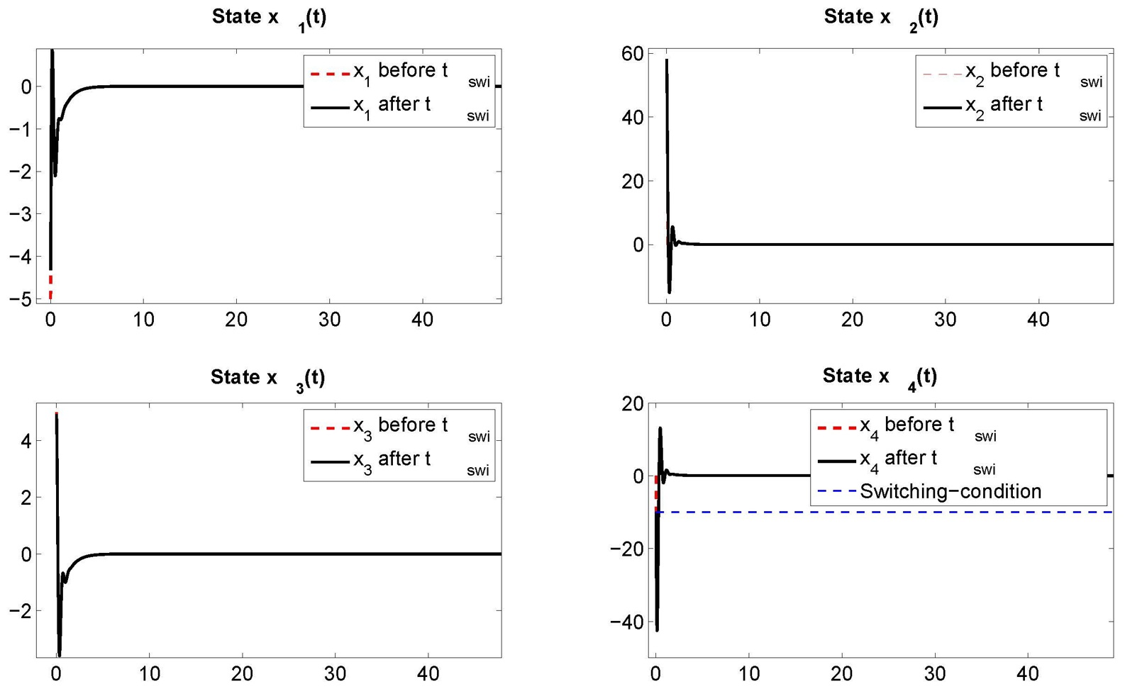
Fig. 2. Components of the optimal trajectories
160
14
Will-be-set-by-IN-TECH
Applications of Nonlinear Control
Finally, let us present the simulation results (figure 2). As we can see, the state x 4 satisfies the
switching condition x 4 + 10 = 0. The computed switching time is equal to tswi = 0.0057 s.
The dynamic behaviour on the second time-interval [0, 50] is presented on the figure (2).
The obtained trajectories of the hybrid states converges to zero. As we can see the dynamic
behaviour of the state vector Xopt( t) generated by the optimal hybrid control uopt( ·) guarantee
a minimal value of the quadratic functional I( ·). This minimal value characterize the specific
control design that guarantee an optimal operation (in the sense of the selected objective) of
the hybrid dynamic system under consideration.
6. Concluding remarks
In this paper we propose new theoretical and computational approaches to a specific class
of hybrid OCPs motivated by general mechanical systems. Using a variational structure
of the nonlinear mechanical systems described by hybrid-type Euler-lagrange or Hamilton
equations, one can formulate an auxiliary problem of multiobjective optimization. This
problem and the corresponding theoretical and numerical techniques from multiobjective
optimization can be effectively applied to numerical solution of the initial hybrid OCP.
The proofs of our results and the consideration of the main numerical concepts are
realized under some differentiability conditions and convexity assumptions. These restrictive
smoothness assumptions are motivated by the "classical" structure of the mechanical hybrid
systems under consideration. On the other hand, the modern variational analysis proceeds
without the above restrictive smoothness assumptions. We refer to [20,21] for theoretical
details. Evidently, the nonsmooth variational analysis and the corresponding optimization
techniques can be considered as a possible mathematical tool for the analysis of discontinuous
(for example, variable structure) and impulsive (nonsmooth) hybrid mechanical systems.
Finally, note that the theoretical approach and the conceptual numerical aspects presented in
this paper can be extended to some constrained OCPs with additional state and/or mixed
constraints. In this case one needs to choose a suitable discretization procedure for the
sophisticated initial OCP and to use the corresponding necessary optimality conditions. It
seems also be possible to apply our theoretical and computational schemes to some practically
motivated nonlinear hybrid and switched OCPs in mechanics, for example, to optimization
problems in robots dynamics.
7. References
[1] R. Abraham, Foundations of Mechanics, WA Benjamin, New York, 1967.
[2] C.D. Aliprantis and K.C. Border, Infinite-Dimensional Analysis, Springer, Berlin, 1999.
[3] V. Azhmyakov and J. Raisch, A gradient-based approach to a class of hybrid optimal
control problems, in: Proceedings of the 2nd IFAC Conference on Analysis and Design of
Hybrid Systems, Alghero, Italy, 2006, pp. 89 – 94.
[4] V. Azhmyakov, S.A. Attia and J. Raisch, On the Maximum Principle for impulsive hybrid
systems, Lecture Notes in Computer Science, vol. 4981, Springer, Berlin, 2008, pp. 30 – 42.
[5] V. Azhmyakov, An approach to controlled mechanical systems based on the
multiobjective technique, Journal of Industrial and Management Optimization, vol. 4, 2008,
pp. 697 – 712
On Optimization Techniques for a Class of Hybrid Mechanical Systems
161
On Optimization Techniques for a Class of Hybrid Mechanical Systems
15
[6] V. Azhmyakov, V.G. Boltyanski and A. Poznyak, Optimal control of impulsive hybrid
systems, Nonlinear Analysis: Hybrid Systems, vol. 2, 2008, pp. 1089 – 1097.
[7] V. Azhmyakov, R. Galvan-Guerra and M. Egerstedt, Hybrid LQ-optimization using
Dynamic Programming, in: Proceedings of the 2009 American Control Conference, St. Louis,
USA, 2009, pp. 3617 – 3623.
[8] V. Azhmyakov, R. Galvan-Guerra and M. Egerstedt, Linear-quadratic optimal control of
hybrid systems: impulsive and non-impulsive models, Automatica, to appear in 2010.
[9] J. Baillieul, The geometry of controlled mechanical systems, in Mathematical Control
Theory (eds. J. Baillieul and J.C. Willems), Springer, New York, 1999, pp. 322 – 354.
[10] A.M. Bloch and P.E. Crouch, Optimal control, optimization and analytical mechanics, in
Mathematical Control Theory (eds. J. Baillieul and J.C. Willems), Springer, New York, 1999,
pp. 268–321.
[11] M.S. Branicky, S.M. Phillips and W. Zhang, Stability of networked control systems:
explicit analysis of delay, in: Proceedings of the 2000 American Control Conference, Chicago,
USA, 2000, pp. 2352 – 2357.
[12] A. Bressan, Impulsive control systems, in Nonsmooth Analysis and Geometric Methods in
Deterministic Optimal Control, (eds. B. Mordukhovich and H.J. Sussmann), Springer, New
York, 1996, pp. 1 – 22.
[13] C. Cassandras, D.L. Pepyne and Y. Wardi, Optimal control of class of hybrid systems,
IEEE Transactions on Automatic Control, vol. 46, no. 3, 2001, pp. 398 – 415.
[14] P.D. Christofides and N.H. El-Farra, Control of Nonlinear and Hybrid Processes, Lecture
notes in Control and Information Sciences, vol. 324, Springer, Berlin, 2005.
[15] F.H. Clarke, Optimization and Nonsmooth Analysis, SIAM, Philadelphia, 1990.
[16] G.P. Crespi, I. Ginchev and M. Rocca, Two approaches toward constrained vector
optimization and identity of the solutions,
Journal of Industrial and Management
Optimization, vol. 1, 2005, pp. 549 – 563.
[17] M. Egerstedt, Y. Wardi and H. Axelsson,
Transition-time optimization for
switched-mode dynamical systems, IEEE Transactions on Automatic Control, vol. 51, no.
1, 2006, pp. 110 – 115.
[18] F.R. Gantmakher, Lectures on Analytical Mechanics (in Russian), Nauka, Moscow, 1966.
[19] D. Liberzon Switching in Systems and Control, Birkhäuser, Boston, 2003.
[20] B.S. Mordukhovich, Variational Analysis and Generalized Differentiation, I: Basic Theory, II
Applications, Springer, New York, 2006.
[21] B.S. Mordukhovich,
Approximation Methods in Problems of Optimization and Optimal
Control, Nauka, Moscow, 1988.
[22] H. Nijmeijer and A.J. Schaft, Nonlinear Dynamical Control Systems, Springer, New York,
1990.
[23] B. Piccoli, Hybrid systems and optimal control, in: Proceedings of the 37th IEEE Conference
on Decision and Control, Tampa, USA, 1998, pp. 13 – 18.
[24] E. Polak, Optimization, Springer, New York, 1997