![]()
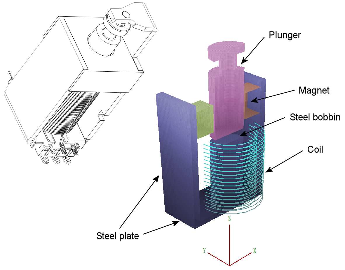
Figure 89: Latching solenoid assembly – drawing and three-dimensional mesh. The parts are displayed in the space y ≥ 0.0 mm and the coil in y ≤ 0.0 mm. The plunger has diameter 10.0 mm and length 28.0 mm.
20 3D magnetic fields: iron and permanent magnets
For the final calculation of the course, we’ll characterize the forces in a latching solenoid. This solution exercises the full finite-element capabilities of Magnum and provides an oppor- tunity to use the force-calculation capabilities of MagView. In preparation, copy the files Latching.CDF, Latching.MIN and Latching.GIN to a working directory and set the Data folder of AMaze. The three input files have the same functions as the ones we encountered in the previous chapter.
Figure 89 shows a drawing of the assembly along with the mesh created by MetaMesh. The neodymium-iron permanent magnets have magnetization directions pointing toward the plunger. They provide a resting holding force to keep the plunger in contact with the steel bobbin. Depending on the polarity of solenoid current, the coil may work in opposition to the permanent magnet to unlatch the plunger or it may assist the permanent magnet to pull in the plunger.
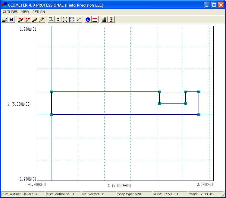
Figure 90: Outline editor showing the outline for the plunger turning.
Run Geometer and load the file Latching.MIN. Check out the script content with the internal editor. A variable-resolution foundation mesh is employed for accurate field calculations at the gap between the bobbin and plunger. The solution includes five physical regions: air, the steel of the case, the steel plunger and the upper and lower magnets. Notice the use of labels and comments to document features of the calculation. Construction of the mesh is straightforward. The Box model is used to represent the steel plates and the magnets, while the bobbin is a Cylinder. The plunger is a Turning, a model we have not yet discussed. A turning is an outline rotated about the z axis of the workbench space. Note the outline vectors in the script following the Type command of the Plunger section.
To see the outline, exit the editor and click Outline. Geometer opens the window of Fig. 90. In contrast to the convention for extrusions, the outline of a turning is defined in cylindrical coordinates, (z, r)19. In the editor, you can modify vectors of the outline using the CAD operations. The changes appear immediately in the Geometer display when you return to the main menu. Changes are recorded if you save the MIN file under the same or a different name. To check the variable mesh definitions, exit the outline editor and click Foundation. The foundation mesh window shows 2D plots of the assembly along with the initial mesh divisions (before fitting). Figure 91 is a zoomed view in a plane normal to the y axis. Note the region of very fine elements (0.025 mm) along z near the gap between the bobbin and plunger. To investigate the holding force of the solenoid, we need to perform surface integrals with very small gaps.
19Vector coordinates of outlines for turnings must satisfy the condition r ≥ 0.0.
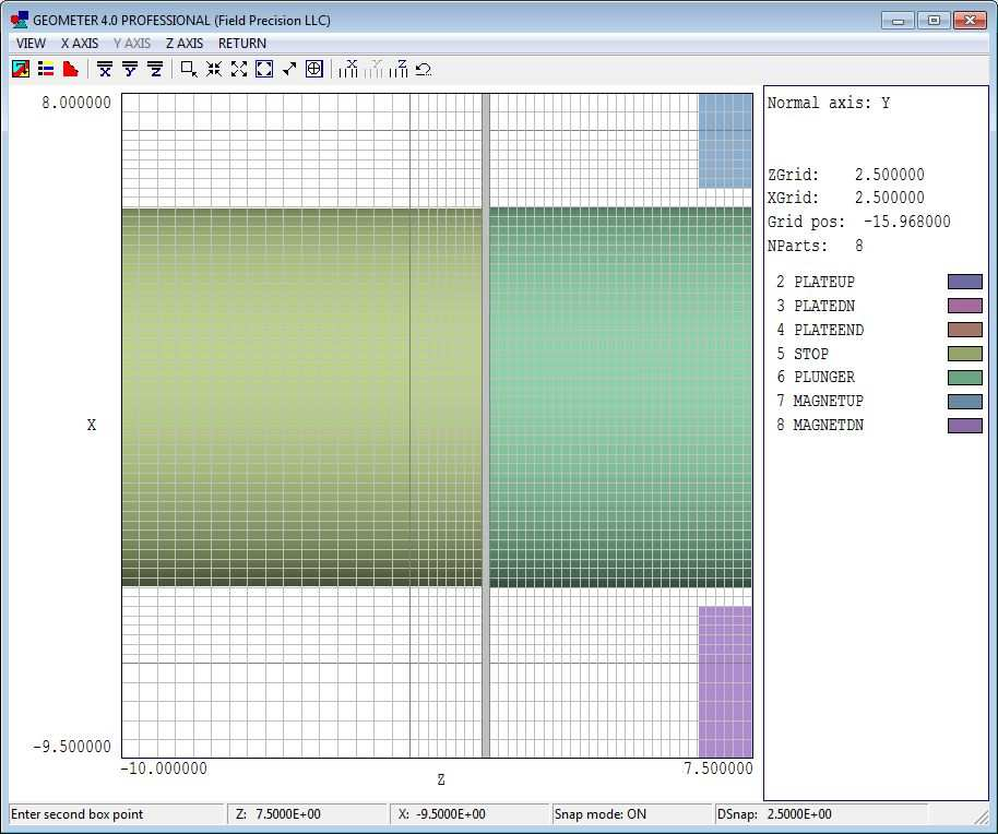
Figure 91: Detailed view of the foundation mesh showing the fine division in z at the bobbin- plunger gap.
Let’s proceed to the solution. Run Magwinder and load Latching.CDF with the content:
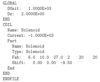
The coil definition file uses the Solenoid model to create 800 applied current elements with a coil current of -1000 A-turn. The negative value gives a coil field inside the bobbin in the same direction as the permanent magnet field. Click File/Save element file to create Latching.WND.
Run MetaMesh and process the MIN file to create Latching.MDF. To check out the con- trols for the finite-element solution, run Magnum, click File/Edit input files and choose Latching.GIN. The file has the following content:
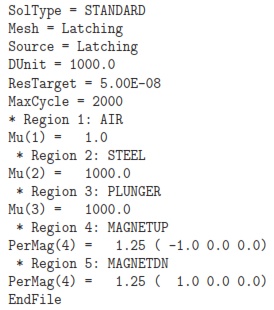
In contrast to the free-space solutions we discussed previously, the solution type is set to Standard and physical characteristics are assigned to the regions. The quantities ResTarget and MaxCycle control the iterative solution of the finite-element equations – default values are usually appropriate. For magnetic-field solutions, material quantities are the relative magnetic permeability and the parameters of permanent magnets. Because we do not expect saturation effects at the device field levels, we assign the high value µr = 1000.0 to the case, bobbin and plunger. The specification of a permanent magnet material includes the remanence field Br = 1.25 tesla and a vector pointing along the direction of magnetization. The magnetization of the top magnet points in the -x direction and the bottom magnet in the +x direction.
Run Magnum to create the output file Latching.GOU. Figure 92 shows the distribution of |B| in the plane y = 0.0 mm with the plunger in contact with the bobbin. The combination of flux from the two magnets produces an approximately uniform field at the contact point of B0 = 1.61 tesla. Note that it is not necessary to surround the assembly with a large external volume because the flux is well-contained in the magnetic circuit.
The goal of the calculation is to find the force on the plunger as a function of the gap width. The force calculation is easy when the plunger is well-separated from the bobbin. Because the plunger is surrounded by air (µr = 1.0) elements, we can apply a surface integral of the Maxwell stress tensor over the plunger facets. The definition of the Maxwell tensor is contained in the configuration file Magview Standard.CFG20. It is useful to take a moment to look at the configuration file (usually contained in the Program folder defined in AMaze). Open the file with an editor. It contains definitions for plot quantities and numerical calculations. This section applies to automatic surface integrals:
20The MagView default configuration file is sufficient for most code users. On the other hand, the program has the flexibility to meet the needs of power users. You can set up custom configuration files with user-defined quantities.
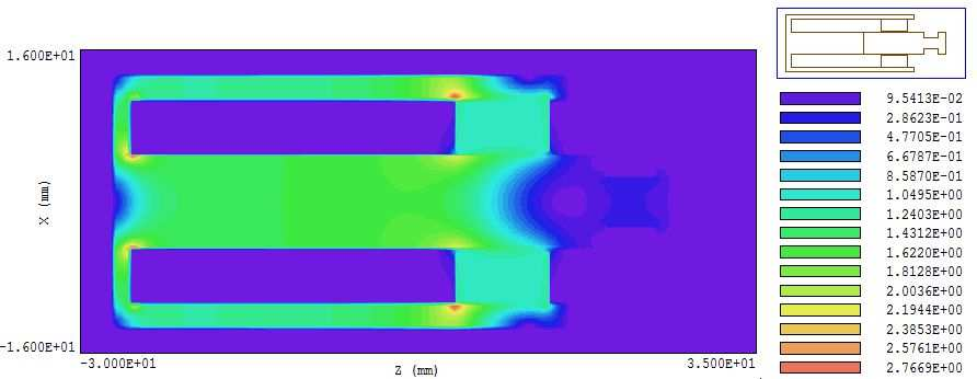
Figure 92: Field distribution in the latched state in the plane y = 0.0 mm. Color-coding shows |B| in tesla.
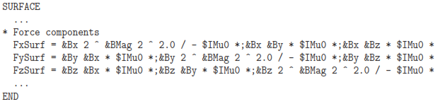
The expressions give the force components determined from the Maxwell integral at a point. Quantities like &Bx are calculated field quantities at the point, while quantities like $IMu0 are defined constants.
Run MagView and load the file Latching.GOU. To find the total force on the plunger, click Analysis/Surface integrals in the main menu to bring up the dialog of Fig. 93. The internal region is the Plunger and the single external region is Air. Click OK and save the results to the file Latching.DAT. Here is the result for a gap width of 0.20 mm with zero coil current:
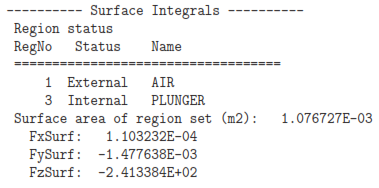
As an indication of accuracy, the force components Fx and Fy (theoretically zero) are smaller than Fz by a factor exceeding 1/100,000. With a gap of 3.0 mm, the axial force with no coil current is Fz = −1.111 N. The force increases to -7.427 N with a coil current of -1000 A-turns.
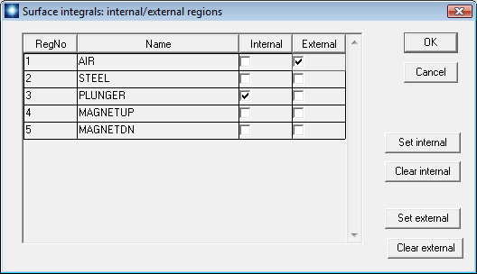
Figure 93: Surface integral dialog. In this case, the integral is taken over all external facets of the plunger in contact with air elements.
A quantity of particular interest is the holding force in the latched state (i.e., plunger touching the bobbin with no coil current). In this case, a Maxwell stress tensor integral around the plunger does not apply because the plunger and bobbin are effectively the same piece of material. One option is to perform a series of calculations with an air gap of decreasing width dg. The goal would be to fit the force variation with an interpolation function extrapolated to dg = 0.0. Figure 94 shows results of such a calculation. A simple plot of Fz versus dg would not be informative because the force varies by orders of magnitude. The strong variation reflects the familiar experience of two magnets snapping together when they are close. A helpful observation is that force scales as 1/d2 for gaps greater than 0.5 mm. Therefore, it is useful to construct a log-log plot of 1/√Fz versus dg. The data of Fig. 94 indicate that the force approaches a constant value at zero spacing. This calculation strategy requires considerable accuracy and effort. It is necessary to include results for very small gap widths (dg = 0.05 mm) to observe the inflection toward a constant value.
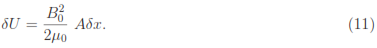
Fortunately, there is a simple way to determine the exact holding force from a knowledge of the flux distribution at dg = 0.0 mm. Suppose we displace the plunger an infinitesimal distance δx from the bobbin. The field in the air gap would remain confined to the cross section area A of steel parts with a value approximately equal to the zero gap field, B0. The change in field energy in the magnet circuit is
Using the principle of virtual work, the holding force is
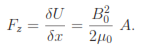 . (12)
With a plunger diameter of 10.0 mm, the area is A = 7.854 × 10 m2. With B0 = 1.61 tesla, the total predicted force is Fz = −80.935 N (plotted as a dashed red line in Fig. 94). The mass equivalent is 8.25 kg.
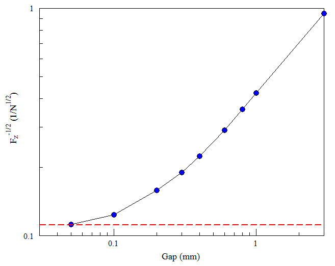
Figure 94: Plot of 1/√Fz as function of the gap between the plunger and the bobbin, where Fz is the force on the plunger in newtons. Blue circles indicate results determined by a MagView surface integral. The dashed red line indicates the theoretical value for zero gap.
We’ve covered a lot of territory in this book. We’ve had a chance to get familiar with the operation sequences and data organization of 2D and 3D programs and discovered many useful analysis techniques. Hopefully, the material will help you get started on your own electric and magnetic field applications. There’s still a lot to discover EStat, PerMag, HiPhi and Magnum have a wealth of capabilities that couldn’t be covered in a short introduction.
To conclude, I’ll list additional resources. First, let’s review materials included with the soft- ware packages. There are individual PDF manuals for Mesh, EStat, PerMag, MetaMesh, HiPhi and Magnum. They serve as comprehensive references through the extensive use of hy- perlinks. The active table of contents is displayed if you activate the bookmark view in your PDF reader. Each manual also has a index with active page links. All software packages include an example library containing ready-to-run, annotated input files for a variety of applications. Be sure to look at text files in the example directories with names like HIPHI EXAMPLE INDEX.TXT. They contain a list of the examples along with a brief description of interesting features.
The following free resources are available on our Internet site:
• Use this link to download a zip archive of input files for the examples discussed in this book: http://www.fieldp.com/freeware/femfield examples.zip.
• Finite-element Methods for Electromagnetics. A full-length text published in 1997 by CRC Press. It reviews the physics of electrostatics and magnetostatics and gives a detailed description of the mechanics of EStat and PerMag. The book is an essential reference if you want to check under the hood to see how finite-element programs work. http://www.fieldp.com/femethods.html
• Field Precision Technical library. This Internet page has downloadable copies of the latest manuals for all Field Precision programs. In addition, there are many tutorials in PDF format that review solution techniques for electric and magnetic field applications. http://www.fieldp.com/library.html
• Field Precision software tips. This blog includes almost 300 articles on finite-element modeling of electromagnetic fields as well as tips on using Windows computers. The best place to start is the index where articles are organized by related software packages. http://fieldp.com/myblog/index-computational-techniques-by-program/