![]()
19 3D magnetic fields: free-space calculations
In this chapter we’ll continue the topic of 3D magnetic fields by discussing Magnum operation in the FreeSpace mode. The mode applies to calculations in an infinite space without magnetic materials. In other words, all objects in the solution space have µr = 1.0. To start, let’s determine the field generated by the set of three solenoid coils that we built in the previous chapter. The end result of that work was the file ReversingSolenoid.WND that contained a set of current elements to approximate the coil set.
The first step in the field solution is to create a mesh. Wait a minute – why do we need a mesh? The previous chapter emphasized that free space calculations used Biot-Savart integrals and had nothing to do with finite-element methods. Here’s the reason. An integral over the full set of current elements involves considerable computational work and gives the magnetic flux density [Bx, By, Bz] at a single point in space. With this approach, it could take several minutes to create a high-resolution plot of field quantities in a plane. Particle tracking, which involves field calculations at thousands of points along the trajectory, would be impossible. It is much more efficient to apply integrals to calculate field values at a given set of points in space (i.e. a mesh), and then to use interpolations to find field values at intervening points. In other words, we do the Biot-Savart integrals once to calculate B values at mesh points, and then we can use the values to make any plots and trajectory calculations we want. Another advantage of recording values on a mesh is that all the Magnum plotting and interpolation routines developed for finite-element calculations can be applied directly.
Fortunately, it takes only a minute or two to make a mesh for a Magnum free-space calculation. All we need is an appropriate set of interpolation points. It is not necessary to make a detailed conformal mesh to represent physical objects17. Run Geometer and choose File/New script. We’ll create an interpolation mesh that encompasses the three coils18. Supply the name ReversingSolenoid and the following dimensions for the solution volume: -5.0 ≤ x ≤ 5.0, 14.0 ≤ y ≤ 24.0, -10.0 ≤ z ≤ 10.0. When you click OK, Geometer sets up the mesh with one default region and part that covers the full volume. Go to the Foundation menu and change the element sizes along each axis to 0.10. Then, save the mesh. Run MetaMesh and process ReversingSolenoid.MIN to create ReversingSolenoid.MDF.
Run Magnum, click Setup and choose ReversingSolenoid.MDF. Figure 83 shows the setup dialog with appropriate settings. Note that the dialog fields associated with finite-element solutions (including the material properties at the bottom) become inactive when you click the Free space radio button. Save the information as ReversingSolenoid.GIN. We now have the three files necessary for the calculation:
17There is considerable flexibility in creating meshes for free-space calculations. You could employ variable resolution for high accuracy in a region. You could even use a conformal mesh if you wanted to represent object boundaries in plots.
18It is important to realize that the size and location of the interpolation mesh has no effect on the field values. You could create a small mesh if you wanted detailed field values within one of the coils.
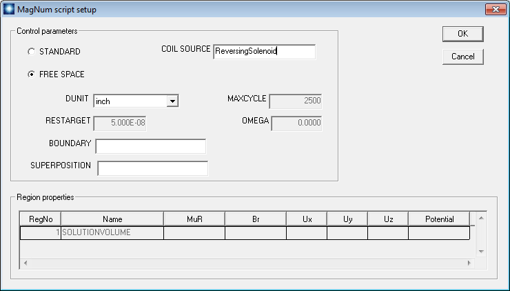
Figure 83: Magnum input dialog for a free-space calculation.
• ReversingSolenoid.CDF: current elements for the Biot-Savart integral.
• ReversingSolenoid.MDF: interpolation points to calculate [Bx, By, Bz].
• ReversingSolenoid.GIN: a short control script to let Magnum know what it’s supposed to do.
In the main Magnum menu, click Run to create the solution file ReversingSolenoid.GOU.
To analyze the results, run MagView, click File/Load solution file and choose the solution. Go to Slice plots and click Slice normal to X. Zoom in to the create the plot of Fig. 84, showing the distribution of |B| in the plane x = 0.0”. MagView has plot and analysis capabilities similar to those of PhiView. For example, we can make a quick check of the magnitude and direction of B with the vector probe. To activate it, click Vector tools/Vector probe and then move the mouse cursor into the plot region. The probe, shown in Fig. 84, points along B. Values of the cursor position and |B| are listed in the status bar at the bottom.
To conclude this chapter, we’ll run through an application example with prepared input files (CathodeHeater.CDF, CathodeHeater.MIN and CathodeHeater.GIN). The goal is to find the magnetic flux density on the surface of a thermionic cathode generated by its heater coil. Figure 85 shows the heater geometry, counter-wound helices with connections and leads. Arrows have been added to show the direction of current. The drive coils are defined in the file CathodeHeater.CDF, listed in Table 4.
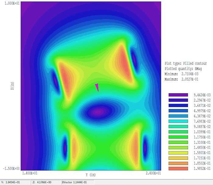
Figure 84: Reversing solenoid example, plot of |B| in the plane x = 0.0”, showing the vector probe.
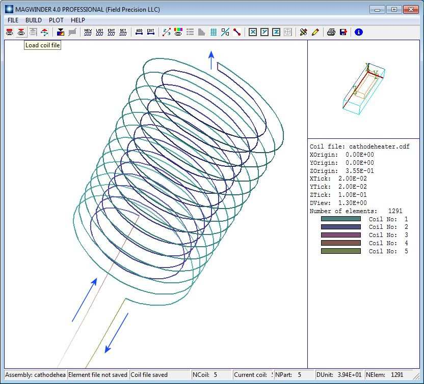
Figure 85: Geometry of the heater coil, arrows added to show the direction of the current.
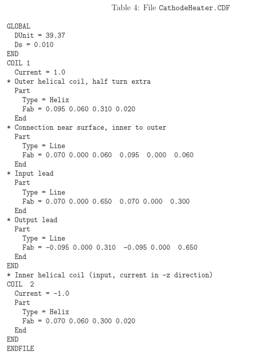
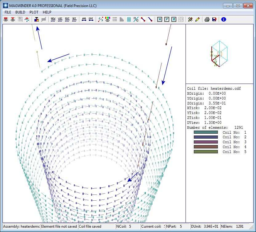
Figure 86: Heater coil, sperm plot option to show the direction of current flow in the elements.
The assembly contains two coils. The first coil, with current 1.0 A, consists of four parts. Three of the parts are straight wires, defined by their start and end points in the assembly space: the input and output leads and the connection between the helical coils. Current always flows from start to end. The Helix model requires four fabrication parameters:
Radius (0.095")
ZStart (0.060")
ZEnd (0.310")
Pitch, or distance between the turns (0.020")
The number of turns equals |ZendZstart|/P itch. The cathode surface is at z = 0.00”, so the distance to the closest part of the coil is 0.060”. Helices always have positive rotation proceeding from Zstart to Zend. To make counter-wound coils, the return helix is contained in its own coil structure with current -1.0 A. For physically-correct results, it’s important that different parts connect to make a continuous coil, and that currents flow in the correct direction. To check validity, you can use the Plot/Sperm plot option in either the 2D or 3D views. Figure 86 shows the result. The elements swim in the direction of the current. In particular, the helix currents are correct with respect to the leads and to each other. Move the example files to a working directory, set the Data folder in Amaze and run MagWinder. Load the coil-definition file and click File/Save element file to create CathodeHeater.WND.
The file CathodeHeater.MIN defines a network of points in space where values of B are calculated from the current elements and recorded. It has the content:
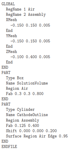
The commands in the Global section create a solution volume that encloses the heater coil and cathode surface. The solution volume part fills the entire solution space. Note that there is an additional region that represents the cylindrical cathode volume. The conformal region has no effect on the calculation of applied fields – it is added to include a reference outline of the cathode in plots. Run MetaMesh, process the mesh and save the file CathodeHeater.MDF.
The file to control the Magnum calculation, CathodeHeater.GIN, is quite simple:
SOLTYPE Free
MESH CathodeHeater
SOURCE CathodeHeater
DUNIT 39.37
ENDFILE
The actions are to load CathodeHeater.WND and CathodeHeater.MDF and to interpret the dimensions in inches. Run Magnum and generate the solution, then run MagView to analyze the results. Figure 87 shows a filled-contour plot of |B| in the plane y = 0.0”. As expected, the magnetic flux is concentrated between the helices. The plot illustrates two special features of MagView slice plots:
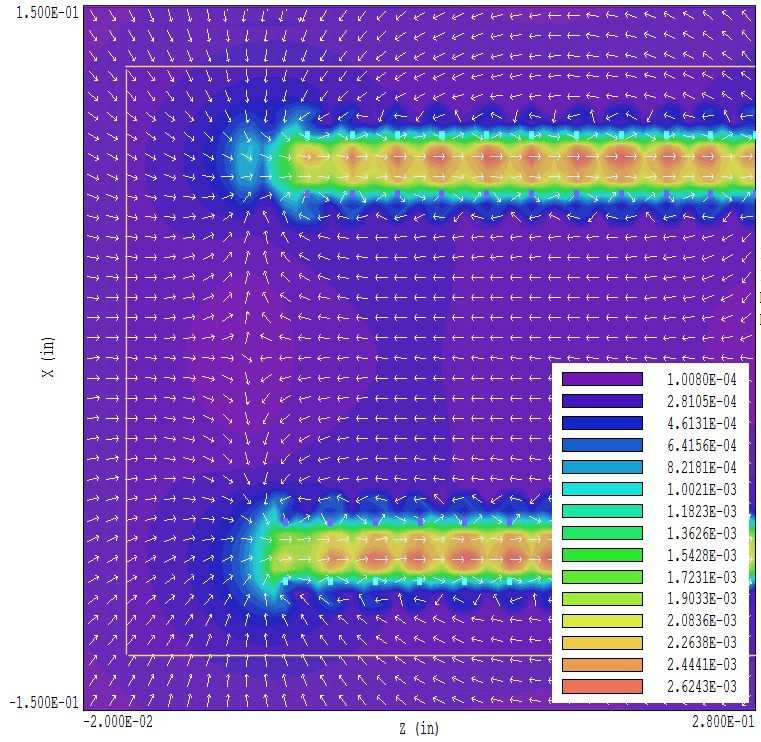
Figure 87: Heater coil, variation of |B| in the plane y = 0.0”. The slice plot shows the intersection points of the helical coils and arrows to designate the direction of B.
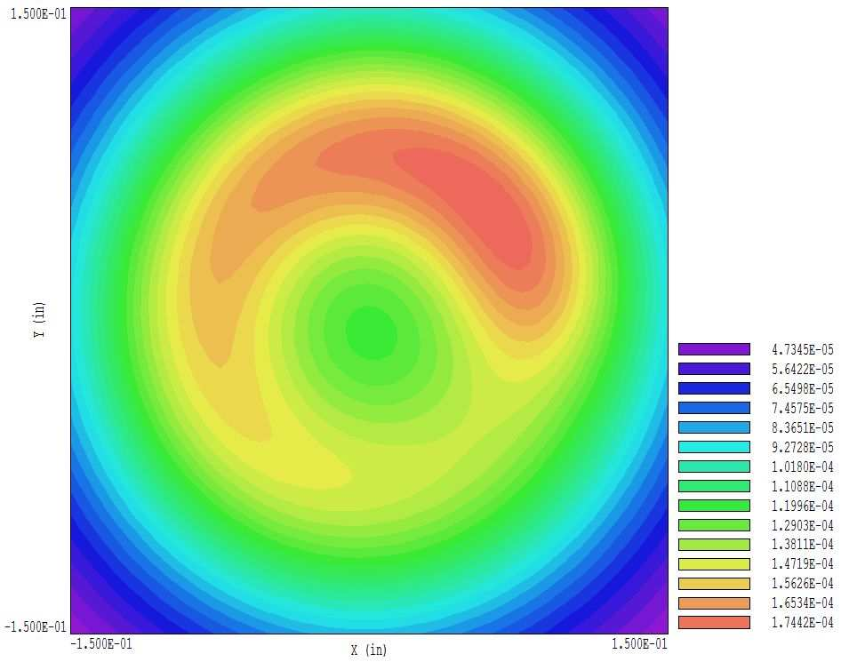
Figure 88: Heater coil, variation of |B| at the cathode surface.
• The drive coils may be superimposed on field plots. The command File/Load coils was used to load CathodeHeater.WND. The intersections of the coil with the plane y = 0.0” are shown as cyan and violet rectangles in the plot.
• Arrows showing the direction of B were added with the command Vector tools/Vector arrow plot.
The cathode boundary is marked by yellow lines. The field at the surface approximates a dipole variation. Finally, Fig. 88 shows a plot of |B| at the cathode surface. The field from the heater configuration approaches 2 Gauss, about 8 times higher than the earth’s field. It would be worthwhile to check alternate heater geometries.