Practice1
by Steven G. Johnson (Department of Mathematics, Massachusetts
Institute of Technology) and Matteo Frigo (Cilk Arts, Inc.)
11.1 Introduction
Although there are a wide range of fast Fourier transform (FFT)
algorithms, involving a wealth of mathematics from number the-
ory to polynomial algebras, the vast majority of FFT implementa-
tions in practice employ some variation on the Cooley-Tukey al-
gorithm [92]. The Cooley-Tukey algorithm can be derived in two
or three lines of elementary algebra. It can be implemented almost
as easily, especially if only power-of-two sizes are desired; numer-
ous popular textbooks list short FFT subroutines for power-of-two
sizes, written in the language du jour. The implementation of the
Cooley-Tukey algorithm, at least, would therefore seem to be a
long-solved problem. In this chapter, however, we will argue that
matters are not as straightforward as they might appear.
1This content is available online at <http://cnx.org/content/m16336/1.15/>.
Available for free at Connexions
<http://cnx.org/content/col10683/1.5>
155
CHAPTER 11. IMPLEMENTING FFTS IN
156
PRACTICE
For many years, the primary route to improving upon the Cooley-
Tukey FFT seemed to be reductions in the count of arithmetic op-
erations, which often dominated the execution time prior to the
ubiquity of fast floating-point hardware (at least on non-embedded
processors). Therefore, great effort was expended towards find-
ing new algorithms with reduced arithmetic counts [114], from
Winograd’s method to achieve Θ (n) multiplications2 (at the cost of
many more additions) [411], [180], [116], [114] to the split-radix
variant on Cooley-Tukey that long achieved the lowest known to-
tal count of additions and multiplications for power-of-two sizes
[422], [107], [391], [230], [114] (but was recently improved upon
[202], [225]). The question of the minimum possible arithmetic
count continues to be of fundamental theoretical interest—it is not
even known whether better than Θ (nlogn) complexity is possible,
since Ω (nlogn) lower bounds on the count of additions have only
been proven subject to restrictive assumptions about the algorithms
[248], [280], [281]. Nevertheless, the difference in the number of
arithmetic operations, for power-of-two sizes n, between the 1965
radix-2 Cooley-Tukey algorithm (∼ 5nlog2n [92]) and the cur-
rently lowest-known arithmetic count (∼ 34 nlog
9
2n [202], [225])
remains only about 25%.
2We employ the standard asymptotic notation of O for asymptotic upper
bounds, Θ for asymptotic tight bounds, and Ω for asymptotic lower bounds
[210].
Available for free at Connexions
<http://cnx.org/content/col10683/1.5>
157
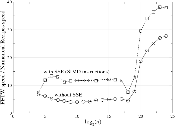
Figure 11.1: The ratio of speed (1/time) between a highly op-
timized FFT (FFTW 3.1.2 [133], [134]) and a typical textbook
radix-2 implementation (Numerical Recipes in C [290]) on a
3 GHz Intel Core Duo with the Intel C compiler 9.1.043, for
single-precision complex-data DFTs of size n, plotted versus
log2n. Top line (squares) shows FFTW with SSE SIMD in-
structions enabled, which perform multiple arithmetic opera-
tions at once (see section ); bottom line (circles) shows FFTW
with SSE disabled, which thus requires a similar number of
arithmetic instructions to the textbook code. (This is not in-
tended as a criticism of Numerical Recipes—simple radix-2
implementations are reasonable for pedagogy—but it illus-
trates the radical differences between straightforward and op-
timized implementations of FFT algorithms, even with simi-
lar arithmetic costs.) For n
219, the ratio increases because
the textbook code becomes much slower (this happens when
the DFT size exceeds the level-2 cache).
And yet there is a vast gap between this basic mathematical theory
and the actual practice—highly optimized FFT packages are often
Available for free at Connexions
<http://cnx.org/content/col10683/1.5>
CHAPTER 11. IMPLEMENTING FFTS IN
158
PRACTICE
an order of magnitude faster than the textbook subroutines, and the
internal structure to achieve this performance is radically different
from the typical textbook presentation of the “same” Cooley-Tukey
algorithm. For example, Figure 11.1 plots the ratio of benchmark
speeds between a highly optimized FFT [133], [134] and a typical
textbook radix-2 implementation [290], and the former is faster
by a factor of 5–40 (with a larger ratio as n grows). Here, we
will consider some of the reasons for this discrepancy, and some
techniques that can be used to address the difficulties faced by a
practical high-performance FFT implementation.3
In particular, in this chapter we will discuss some of the lessons
learned and the strategies adopted in the FFTW library. FFTW
[133], [134] is a widely used free-software library that computes
the discrete Fourier transform (DFT) and its various special cases.
Its performance is competitive even with manufacturer-optimized
programs [134], and this performance is portable thanks the struc-
ture of the algorithms employed, self-optimization techniques,
and highly optimized kernels (FFTW’s codelets) generated by a
special-purpose compiler.
This chapter is structured as follows. First "Review of the Cooley-
Tukey FFT" (Section 11.2: Review of the Cooley-Tukey FFT),
we briefly review the basic ideas behind the Cooley-Tukey algo-
rithm and define some common terminology, especially focusing
on the many degrees of freedom that the abstract algorithm al-
lows to implementations. Next, in "Goals and Background of the
FFTW Project" (Section 11.3: Goals and Background of the FFTW
Project), we provide some context for FFTW’s development and
stress that performance, while it receives the most publicity, is not
necessarily the most important consideration in the implementa-
3We won’t address the question of parallelization on multi-processor ma-
chines, which adds even greater difficulty to FFT implementation—although
multi-processors are increasingly important, achieving good serial performance is a basic prerequisite for optimized parallel code, and is already hard enough!
Available for free at Connexions
<http://cnx.org/content/col10683/1.5>
159
tion of a library of this sort. Third, in "FFTs and the Memory
Hierarchy" (Section 11.4: FFTs and the Memory Hierarchy), we
consider a basic theoretical model of the computer memory hierar-
chy and its impact on FFT algorithm choices: quite general consid-
erations push implementations towards large radices and explicitly
recursive structure. Unfortunately, general considerations are not
sufficient in themselves, so we will explain in "Adaptive Compo-
sition of FFT Algorithms" (Section 11.5: Adaptive Composition
of FFT Algorithms) how FFTW self-optimizes for particular ma-
chines by selecting its algorithm at runtime from a composition
of simple algorithmic steps. Furthermore, "Generating Small FFT
Kernels" (Section 11.6: Generating Small FFT Kernels) describes
the utility and the principles of automatic code generation used to
produce the highly optimized building blocks of this composition,
FFTW’s codelets. Finally, we will briefly consider an important
non-performance issue, in "Numerical Accuracy in FFTs" (Sec-
tion 11.7: Numerical Accuracy in FFTs).
11.2 Review of the Cooley-Tukey FFT
The (forward, one-dimensional) discrete Fourier transform (DFT)
of an array X of n complex numbers is the array Y given by
n−1
Y [k] =
k
∑ X [ ] ωn ,
(11.1)
=0
where 0 ≤ k < n and ωn = exp (−2πi/n) is a primitive root of
unity. Implemented directly, (11.1) would require Θ n2 opera-
tions; fast Fourier transforms are O (nlogn) algorithms to compute
the same result. The most important FFT (and the one primarily
used in FFTW) is known as the “Cooley-Tukey” algorithm, after
the two authors who rediscovered and popularized it in 1965 [92],
although it had been previously known as early as 1805 by Gauss
as well as by later re-inventors [173]. The basic idea behind this
Available for free at Connexions
<http://cnx.org/content/col10683/1.5>
CHAPTER 11. IMPLEMENTING FFTS IN
160
PRACTICE
FFT is that a DFT of a composite size n = n1n2 can be re-expressed
in terms of smaller DFTs of sizes n1 and n2—essentially, as a two-
dimensional DFT of size n1 × n2 where the output is transposed.
The choices of factorizations of n, combined with the many differ-
ent ways to implement the data re-orderings of the transpositions,
have led to numerous implementation strategies for the Cooley-
Tukey FFT, with many variants distinguished by their own names
[114], [389]. FFTW implements a space of many such variants,
as described in "Adaptive Composition of FFT Algorithms" (Sec-
tion 11.5: Adaptive Composition of FFT Algorithms), but here we
derive the basic algorithm, identify its key features, and outline
some important historical variations and their relation to FFTW.
The Cooley-Tukey algorithm can be derived as follows. If n can
be factored into n = n1n2, (11.1) can be rewritten by letting
=
1n2 + 2 and k = k1 + k2n1. We then have:
Y [k
n2−1
n1−1
1 + k2n1] = ∑
X [ 1n2 + 2] ω 1k1
n
ω 2k1
n
(11.2)
ω 2k2
n
,
2=0
∑ 1=0
1
2
where k1,2 = 0, ..., n1,2 − 1. Thus, the algorithm computes n2 DFTs
of size n1 (the inner sum), multiplies the result by the so-called
[139] twiddle factors ω 2k1
n
, and finally computes n1 DFTs of size
n2 (the outer sum). This decomposition is then continued recur-
sively. The literature uses the term radix to describe an n1 or n2
that is bounded (often constant); the small DFT of the radix is tra-
ditionally called a butterfly.
Many well-known variations are distinguished by the radix alone.
A decimation in time (DIT) algorithm uses n2 as the radix, while
a decimation in frequency (DIF) algorithm uses n1 as the radix.
If multiple radices are used, e.g. for n composite but not a prime
power, the algorithm is called mixed radix. A peculiar blending of
radix 2 and 4 is called split radix, which was proposed to minimize
the count of arithmetic operations [422], [107], [391], [230], [114]
Available for free at Connexions
<http://cnx.org/content/col10683/1.5>
161
although it has been superseded in this regard [202], [225]. FFTW
implements both DIT and DIF, is mixed-radix with radices that
are adapted to the hardware, and often uses much larger radices
(e.g. radix 32) than were once common. On the other end of the
√
scale, a “radix” of roughly
n has been called a four-step FFT al-
gorithm (or six-step, depending on how many transposes one per-
forms) [14]; see "FFTs and the Memory Hierarchy" (Section 11.4:
FFTs and the Memory Hierarchy) for some theoretical and practi-
cal discussion of this algorithm.
A key difficulty in implementing the Cooley-Tukey FFT is that the
n1 dimension corresponds to discontiguous inputs 1 in X but con-
tiguous outputs k1 in Y, and vice-versa for n2. This is a matrix
transpose for a single decomposition stage, and the composition of
all such transpositions is a (mixed-base) digit-reversal permutation
(or bit-reversal, for radix 2). The resulting necessity of discon-
tiguous memory access and data re-ordering hinders efficient use
of hierarchical memory architectures (e.g., caches), so that the op-
timal execution order of an FFT for given hardware is non-obvious,
and various approaches have been proposed.
Available for free at Connexions
<http://cnx.org/content/col10683/1.5>
CHAPTER 11. IMPLEMENTING FFTS IN
162
PRACTICE
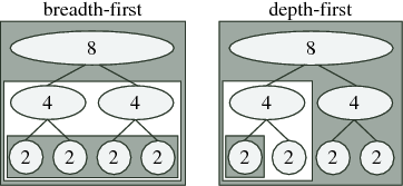
Figure 11.2: Schematic of traditional breadth-first (left) vs.
recursive depth-first (right) ordering for radix-2 FFT of size
8: the computations for each nested box are completed be-
fore doing anything else in the surrounding box. Breadth-
first computation performs all butterflies of a given size at
once, while depth-first computation completes one subtrans-
form entirely before moving on to the next (as in the algorithm
below).
One ordering distinction is between recursion and iteration. As ex-
pressed above, the Cooley-Tukey algorithm could be thought of as
defining a tree of smaller and smaller DFTs, as depicted in Fig-
ure 11.2; for example, a textbook radix-2 algorithm would divide
size n into two transforms of size n/2, which are divided into four
transforms of size n/4, and so on until a base case is reached (in
principle, size 1). This might naturally suggest a recursive im-
plementation in which the tree is traversed “depth-first” as in Fig-
ure 11.2(right) and the algorithm of p. ??—one size n/2 transform
is solved completely before processing the other one, and so on.
However, most traditional FFT implementations are non-recursive
(with rare exceptions [341]) and traverse the tree “breadth-first”
[389] as in Figure 11.2(left)—in the radix-2 example, they would
perform n (trivial) size-1 transforms, then n/2 combinations into
Available for free at Connexions
<http://cnx.org/content/col10683/1.5>
163
size-2 transforms, then n/4 combinations into size-4 transforms,
and so on, thus making log2n passes over the whole array. In con-
trast, as we discuss in "Discussion" (Section 11.5.2.6: Discussion), FFTW employs an explicitly recursive strategy that encompasses
both depth-first and breadth-first styles, favoring the former since
it has some theoretical and practical advantages as discussed in
"FFTs and the Memory Hierarchy" (Section 11.4: FFTs and the
Memory Hierarchy).
Y [0, ..., n − 1] ← rec f f t 2 (n, X, ι )✿
■❋ ♥❂✶ ❚❍❊◆
Y [0] ← X [0]
❊▲❙❊
Y [0, ..., n/2 − 1] ← rec f f t2 (n/2, X, 2ι )
Y [n/2, ..., n − 1] ← rec f f t2 (n/2, X + ι , 2ι )
❋❖❘ k❴1 = 0 ❚❖ (n/2) − 1 ❉❖
t ← Y [k❴1]
Y [k❴1] ← t + ω ❴nˆk❴1Y [k❴1 + n/2]
Y [k❴1 + n/2] ← t − ω ❴nˆk❴1Y [k❴1 + n/2]
❊◆❉ ❋❖❘
❊◆❉ ■❋
Listing 11.1: A depth-first recursive radix-2 DIT Cooley-
Tukey FFT to compute a DFT of a power-of-two size n = 2m.
The input is an array X of length n with stride ι (i.e., the inputs
are X [ ι] for
= 0, ..., n − 1) and the output is an array Y of
length n (with stride 1), containing the DFT of X [Equation 1].
X + ι denotes the array beginning with X [ι]. This algorithm
operates out-of-place, produces in-order output, and does not
require a separate bit-reversal stage.
Available for free at Connexions
<http://cnx.org/content/col10683/1.5>
CHAPTER 11. IMPLEMENTING FFTS IN
164
PRACTICE
A second ordering distinction lies in how the digit-reversal is per-
formed. The classic approach is a single, separate digit-reversal
pass following or preceding the arithmetic computations; this ap-
proach is so common and so deeply embedded into FFT lore that
many practitioners find it difficult to imagine an FFT without an
explicit bit-reversal stage. Although this pass requires only O (n)
time [207], it can still be non-negligible, especially if the data is
out-of-cache; moreover, it neglects the possibility that data reorder-
ing during the transform may improve memory locality. Perhaps
the oldest alternative is the Stockham auto-sort FFT [367], [389],
which transforms back and forth between two arrays with each but-
terfly, transposing one digit each time, and was popular to improve
contiguity of access for vector computers [372]. Alternatively, an
explicitly recursive style, as in FFTW, performs the digit-reversal
implicitly at the “leaves” of its computation when operating out-of-
place (see section "Discussion" (Section 11.5.2.6: Discussion)). A
simple example of this style, which computes in-order output using
an out-of-place radix-2 FFT without explicit bit-reversal, is shown
in the algorithm of p. ?? [corresponding to Figure 11.2(right)].
To operate in-place with O (1) scratch storage, one can interleave
small matrix transpositions with the butterflies [195], [375], [297],
[166], and a related strategy in FFTW [134] is briefly described by
"Discussion" (Section 11.5.2.6: Discussion).
Finally, we should mention that there are many FFTs entirely dis-
tinct from Cooley-Tukey. Three notable such algorithms are the
prime-factor algorithm for gcd (n1, n2) = 1 [278], along with
Rader’s [309] and Bluestein’s [35], [305], [278] algorithms for
prime n. FFTW implements the first two in its codelet generator for
hard-coded n "Generating Small FFT Kernels" (Section 11.6: Gen-
erating Small FFT Kernels) and the latter two for general prime n
(sections "Plans for prime sizes" (Section 11.5.2.5: Plans for prime sizes) and "Goals and Background of the FFTW Project" (Section 11.3: Goals and Background of the FFTW Project)). There
is also the Winograd FFT [411], [180], [116], [114], which mini-
Available for free at Connexions
<http://cnx.org/content/col10683/1.5>
165
mizes the number of multiplications at the expense of a large num-
ber of additions; this trade-off is not beneficial on current proces-
sors that have specialized hardware multipliers.
11.3 Goals and Background of the FFTW
Project
The FFTW project, begun in 1997 as a side project of the au-
thors Frigo and Johnson as graduate students at MIT, has gone
through several major revisions, and as of 2008 consists of more
than 40,000 lines of code. It is difficult to measure the popularity
of a free-software package, but (as of 2008) FFTW has been cited
in over 500 academic papers, is used in hundreds of shipping free
and proprietary software packages, and the authors have received
over 10,000 emails from users of the software. Most of this chap-
ter focuses on performance of FFT implementations, but FFTW
would probably not be where it is today if that were the only con-
sideration in its design. One of the key factors in FFTW’s success
seems to have been its flexibility in addition to its performance. In
fact, FFTW is probably the most flexible DFT library available:
• FFTW is written in portable C and runs well on many archi-
tectures and operating systems.
• FFTW computes DFTs in O (nlogn) time for any length n.
(Most other DFT implementations are either restricted to a
subset of sizes or they become Θ n2 for certain values of n,
for example when n is prime.)
• FFTW imposes no restrictions on the rank (dimensionality)
of multi-dimensional transforms. (Most other implementa-
tions are limited to one-dimensional, or at most two- and
three-dimensional data.)
• FFTW supports multiple and/or strided DFTs; for exam-
ple, to transform a 3-component vector field or a portion of
Available for free at Connexions
<http://cnx.org/content/col10683/1.5>
CHAPTER 11. IMPLEMENTING FFTS IN
166
PRACTICE
a multi-dimensional array. (Most implementations support
only a single DFT of contiguous data.)
• FFTW supports DFTs of real data, as well as of real
symmetric/anti-symmetric data (also called discrete co-
sine/sine transforms).
Our design philosophy has been to first define the most general
reasonable functionality, and then to obtain the highest possible
performance without sacrificing this generality. In this section, we
offer a few thoughts about why such flexibility has proved impor-
tant, and how it came about that FFTW was designed in this way.
FFTW’s generality is partly a consequence of the fact the FFTW
project was started in response to the needs of a real application
for one of the authors (a spectral solver for Maxwell’s equations
[204]), which from the beginning had to run on heterogeneous
hardware. Our initial application required multi-dimensional DFTs
of three-component vector fields (magnetic fields in electromag-
netism), and so right away this meant: (i) multi-dimensional FFTs;
(ii) user-accessible loops of FFTs of discontiguous data; (iii) effi-
cient support for non-power-of-two sizes (the factor of eight differ-
ence between n × n × n and 2n × 2n × 2n was too much to tolerate);
and (iv) saving a factor of two for the common real-input case was
desirable. That is, the initial requirements already encompassed
most of the features above, and nothing about this application is
particularly unusual.
Even for one-dimensional DFTs, there is a common mispercep-
tion that one should always choose power-of-two sizes if one cares
about efficiency. Thanks to FFTW’s code generator (described in
"Generating Small FFT Kernels" (Section 11.6: Generating Small
FFT Kernels)), we could afford to devote equal optimization ef-
fort to any n with small factors (2, 3, 5, and 7 are good), instead
of mostly optimizing powers of two like many high-performance
FFTs.
As a result, to pick a typical example on the 3 GHz
Core Duo processor of Figure 11.1, n = 3600 = 24 · 32 · 52 and
Available for free at Connexions
<http://cnx.org/content/col10683/1.5>
167
n = 3840 = 28 · 3 · 5 both execute faster than n = 4096 = 212. (And
if there are factors one particularly cares about, one can generate
code for them too.)
One initially missing feature was efficient support for large prime
sizes; the conventional wisdom was that large-prime algorithms
were mainly of academic interest, since in real applications (in-
cluding ours) one has enough freedom to choose a highly compos-
ite transform size. However, the prime-size algorithms are fasci-
nating, so we implemented Rader’s O (nlogn) prime-n algorithm
[309] purely for fun, including it in FFTW 2.0 (released in 1998)
as a bonus feature. The response was astonishingly positive—
even though users are (probably) never forced by their application
to compute a prime-size DFT, it is rather inconvenient to always
worry that collecting an unlucky number of data points will slow
down one’s analysis by a factor of a million. The prime-size algo-
rithms are certainly slower than algorithms for nearby composite
sizes, but in interactive data-analysis situations the difference be-
tween 1 ms and 10 ms means little, while educating users to avoid
large prime factors is hard.
Another form of flexibility that deserves comment has to do with a
purely technical aspect of computer software. FFTW’s implemen-
tation involves some unusual language choices internally (the FFT-
kernel generator, described in "Generating Small FFT Kernels"
(Section 11.6: Generating Small FFT Kernels), is written in Objec-
tive Caml, a functional language especially suited for compiler-like
programs), but its user-callable inte