The publication by Cooley and Tukey 5 in 1965 of an efficient algorithm for the calculation of the DFT was a major turning point in the development of digital signal processing. During the five or so years that followed, various extensions and modifications were made to the original algorithm 4. By the early 1970's the practical programs were basically in the form used today. The standard development presented in 21, 22, 2 shows how the DFT of a length-N sequence can be simply calculated from the two length-N/2 DFT's of the even index terms and the odd index terms. This is then applied to the two half-length DFT's to give four quarter-length DFT's, and repeated until N scalars are left which are the DFT values. Because of alternately taking the even and odd index terms, two forms of the resulting programs are called decimation-in-time and decimation-in-frequency. For a length of 2M, the dividing process is repeated M=log2N times and requires N multiplications each time. This gives the famous formula for the computational complexity of the FFT of Nlog2N which was derived in Multidimensional Index Mapping: Equation 34.
Although the decimation methods are straightforward and easy to understand, they do not generalize well. For that reason it will be assumed that the reader is familiar with that description and this chapter will develop the FFT using the index map from Multidimensional Index Mapping.
The Cooley-Tukey FFT always uses the Type 2 index map from Multidimensional Index Mapping: Equation 11. This is necessary for the most popular forms that have N=RM, but is also used even when the factors are relatively prime and a Type 1 map could be used. The time and frequency maps from Multidimensional Index Mapping: Equation 6 and Multidimensional Index Mapping: Equation 12 are


Type-2 conditions Multidimensional Index Mapping: Equation 8 and Multidimensional Index Mapping: Equation 11 become

and

The row and column calculations in Multidimensional Index Mapping: Equation 15 are uncoupled by Multidimensional Index Mapping: Equation 16 which for this case are

To make each short sum a DFT, the Ki must satisfy

In order to have the smallest values for Ki the constants in Equation 9.3 are chosen to be
which makes the index maps of Equation 9.1 become
These index maps are all evaluated modulo N, but in Equation 9.8, explicit reduction is not necessary since n never exceeds N. The reduction notation will be omitted for clarity. From Multidimensional Index Mapping: Equation 15 and example Multidimensional Index Mapping: Equation 19, the DFT is

This map of Equation 9.8 and the form of the DFT in Equation 9.10 are the fundamentals of the Cooley-Tukey FFT.
The order of the summations using the Type 2 map in Equation 9.10 cannot be reversed as it can with the Type-1 map. This is because of the WN terms, the twiddle factors.
Turning Equation 9.10 into an efficient program requires some care.
From Multidimensional Index Mapping: Efficiencies Resulting from Index Mapping with the DFT we know that all the factors should be
equal. If
N=RM ,
with R called the radix,
N1
is first set
equal to
R
and
N2
is then necessarily RM–1.
Consider
n1
to be the index along the rows and n2 along the columns. The inner
sum of Equation 9.10 over n1 represents a length-N1 DFT for each value
of n2. These N2 length-N1 DFT's are the DFT's of the rows
of the  array. The resulting array of row DFT's is
multiplied by an array of twiddle factors which are the WN terms
in Equation 9.10. The twiddle-factor array for a length-8 radix-2 FFT
is
array. The resulting array of row DFT's is
multiplied by an array of twiddle factors which are the WN terms
in Equation 9.10. The twiddle-factor array for a length-8 radix-2 FFT
is

The twiddle factor array will always have unity in the first row and first column.
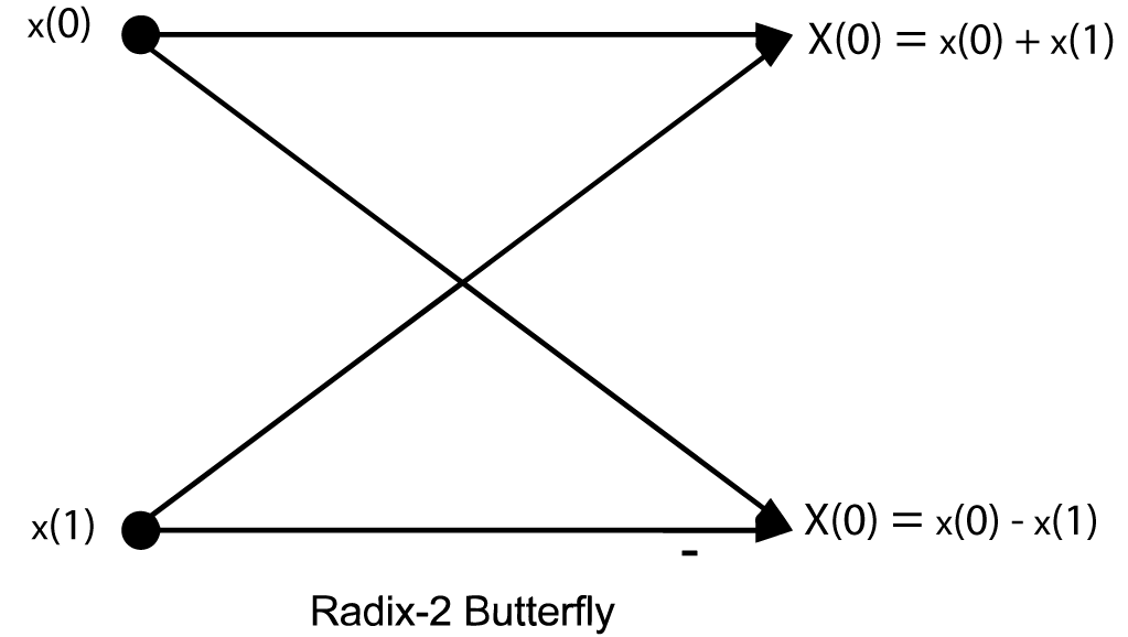
To complete Equation 9.10 at this point, after the row DFT's are multiplied by the TF array, the N1 length-N2 DFT's of the columns are calculated. However, since the columns DFT's are of length RM–1, they can be posed as a RM–2 by R array and the process repeated, again using length-R DFT's. After M stages of length-R DFT's with TF multiplications interleaved, the DFT is complete. The flow graph of a length-2 DFT is given in Figure 1 and is called a butterfly because of its shape. The flow graph of the complete length-8 radix-2 FFT is shown in Figure 2 .

This flow-graph, the twiddle factor map of Equation 9.11, and the basic equation Equation 9.10 should be completely understood before going further.
A very efficient indexing scheme has evolved over the years that results in a compact and efficient computer program. A FORTRAN program is given below that implements the radix-2 FFT. It should be studied 1 to see how it implements Equation 9.10 and the flow-graph representation.
N2 = N
        DO 10 K = 1, M
            N1 = N2
            N2 = N2/2
            E  = 6.28318/N1
            A  = 0
            DO 20 J = 1, N2
                C = COS (A)
                S =-SIN (A)
                A = J*E
                DO 30 I = J, N, N1
                    L = I + N2
                    XT   = X(I) - X(L)
                    X(I) = X(I) + X(L)
                    YT   = Y(I) - Y(L)
                    Y(I) = Y(I) + Y(L)
                    X(L) = XT*C - YT*S
                    Y(L) = XT*S + YT*C
   30           CONTINUE
   20       CONTINUE
   10   CONTINUE
This discussion, the flow graph of Winograd’s Short DFT Algorithms: Figure 2 and the program of screen are all based on the input index map of Multidimensional Index Mapping: Equation 6 and Equation 9.1 and the calculations are performed in-place. According to Multidimensional Index Mapping: In-Place Calculation of the DFT and Scrambling, this means the output is scrambled in bit-reversed order and should be followed by an unscrambler to give the DFT in proper order. This formulation is called a decimation-in-frequency FFT 21, 22, 2. A very similar algorithm based on the output index map can be derived which is called a decimation-in-time FFT. Examples of FFT programs are found in 1 and in the Appendix of this book.
Soon after the paper by Cooley and Tukey, there were improvements and extensions made. One very important discovery was the improvement in efficiency by using a larger radix of 4, 8 or even 16. For example, just as for the radix-2 butterfly, there are no multiplications required for a length-4 DFT, and therefore, a radix-4 FFT would have only twiddle factor multiplications. Because there are half as many stages in a radix-4 FFT, there would be half as many multiplications as in a radix-2 FFT. In practice, because some of the multiplications are by unity, the improvement is not by a factor of two, but it is significant. A radix-4 FFT is easily developed from the basic radix-2 structure by replacing the length-2 butterfly by a length-4 butterfly and making a few other modifications. Programs can be found in 1 and operation counts will be given in "Evaluation of the Cooley-Tukey FFT Algorithms".
Increasing the radix to 8 gives some improvement but not as much as from 2 to 4. Increasing it to 16 is theoretically promising but the small decrease in multiplications is somewhat offset by an increase in additions and the program becomes rather long. Other radices are not attractive because they generally require a substantial number of multiplications and additions in the butterflies.
The second method of reducing arithmetic is to remove the unnecessary TF multiplications by plus or minus unity or by plus or minus the square root of minus one. This occurs when the exponent of WN is zero or a multiple of N/4. A reduction of additions as well as multiplications is achieved by removing these extraneous complex multiplications since a complex multiplication requires at least two real additions. In a program, this reduction is usually achieved by having special butterflies for the cases where the TF is one or j. As many as four special butterflies may be necessary to remove all unnecessary arithmetic, but in many cases there will be no practical improvement above two or three.
In addition to removing multiplications by one or j, there can be a reduction in multiplications by using a special butterfly for TFs with WN/8, which have equal real and imaginary parts. Also, for computers or hardware with multiplication considerably slower than addition, it is desirable to use an algorithm for complex multiplication that requires three multiplications and three additions rather than the conventional four multiplications and two additions. Note that this gives no reduction in the total number of arithmetic operations, but does give a trade of multiplications for additions. This is one reason not to use complex data types in programs but to explicitly program complex arithmetic.
A time-consuming and unnecessary part of the execution of a FFT program is the calculation of the sine and cosine terms which are the real and imaginary parts of the TFs. There are basically three approaches to obtaining the sine and cosine values. They can be calculated as needed which is what is done in the sample program above. One value per stage can be calculated and the others recursively calculated from those. That method is fast but suffers from accumulated round-off errors. The fastest method is to fetch precalculated values from a stored table. This has the disadvantage of requiring considerable memory space.
If all the N DFT values are not needed, special forms of the FFT can be developed using a process called pruning 17 which removes the operations concerned with the unneeded outputs.
Special algorithms are possible for cases with real data or with symmetric data 6. The decimation-in-time algorithm can be easily modified to transform real data and save half the arithmetic required for complex data 27. There are numerous other modifications to deal with special hardware considerations such as an array processor or a special microprocessor such as the Texas Instruments TMS320. Examples of programs that deal with some of these items can be found in 22, 1, 6.
Recently several papers 18, 7, 28, 23, 8 have been published on algorithms to calculate a length-2M DFT more efficiently than a Cooley-Tukey FFT of any radix. They all have the same computational complexity and are optimal for lengths up through 16 and until recently was thought to give the best total add-multiply count possible for any power-of-two length. Yavne published an algorithm with the same computational complexity in 1968 29, but it went largely unnoticed. Johnson and Frigo have recently reported the first improvement in almost 40 years 15. The reduction in total operations is only a few percent, but it is a reduction.
The basic idea behind the split-radix FFT (SRFFT) as derived by Duhamel and Hollmann 7, 8 is the application of a radix-2 index map to the even-indexed terms and a radix-4 map to the odd- indexed terms. The basic definition of the DFT

with W=e–j2π/N gives

for the even index terms, and

and

for the odd index terms. This results in an L-shaped “butterfly" shown in Figure 9.3 which relates a length-N DFT to one length-N/2 DFT and two length-N/4 DFT's with twiddle factors. Repeating this process for the half and quarter length DFT's until scalars result gives the SRFFT algorithm in much the same way the decimation-in-frequency radix-2 Cooley-Tukey FFT is derived 21, 22, 2. The resulting flow graph for the algorithm calculated in place looks like a radix-2 FFT except for the location of the twiddle factors. Indeed, it is the location of the twiddle factors that makes this algorithm use less arithmetic. The L- shaped SRFFT butterfly Figure 9.3 advances the calculation of the top half by one of the M stages while the lower half, like a radix-4 butterfly, calculates two stages at once. This is illustrated for N=8 in Figure 9.4.


Unlike the fixed radix, mixed radix or variable radix Cooley-Tukey FFT or even the prime factor algorithm or Winograd Fourier transform algorithm , the Split-Radix FFT does not progress completely stage by stage, or, in terms of indices, does not complete each nested sum in order. This is perhaps better seen from the polynomial formulation of Martens 18. Because of this, the indexing is somewhat more complicated than the conventional Cooley-Tukey program.
A FORTRAN program is given below which implements the basic decimation-in-frequency split-radix FFT algorithm. The indexing scheme 23 of this program gives a structure very similar to the Cooley-Tukey programs in 1 and allows the same modifications and improvements such as decimation-in-time, multiple butterflies, table look-up of sine and cosine values, three real per complex multiply methods, and real data versions 8, 27.
SUBROUTINE FFT(X,Y,N,M)
        N2 = 2*N
        DO  10 K = 1, M-1
            N2 = N2/2
            N4 = N2/4
            E  = 6.283185307179586/N2
            A = 0
            DO  20 J = 1, N4
                A3  = 3*A
                CC1 = COS(A)
                SS1 = SIN(A)
                CC3 = COS(A3)
                SS3 = SIN(A3)
                A   = J*E
                IS  = J
                ID  = 2*N2
 40             DO 30 I0 = IS, N-1, ID
                    I1 = I0 + N4
                    I2 = I1 + N4
                    I3 = I2 + N4
                    R1    = X(I0) - X(I2)
                    X(I0) = X(I0) + X(I2)
                    R2    = X(I1) - X(I3)
                    X(I1) = X(I1) + X(I3)
                    S1    = Y(I0) - Y(I2)
                    Y(I0) = Y(I0) + Y(I2)
                    S2    = Y(I1) - Y(I3)
                    Y(I1) = Y(I1) + Y(I3)
                    S3    = R1 - S2
                    R1    = R1 + S2
                    S2    = R2 - S1
                    R2    = R2 + S1
                    X(I2) = R1*CC1 - S2*SS1
                    Y(I2) =-S2*CC1 - R1*SS1
                    X(I3) = S3*CC3 + R2*SS3
                    Y(I3) = R2*CC3 - S3*SS3
 30             CONTINUE
                IS = 2*ID - N2 + J
                ID = 4*ID
                IF (IS.LT.N) GOTO 40
 20         CONTINUE
 10     CONTINUE
        IS = 1
        ID = 4
 50     DO 60 I0 = IS, N, ID
            I1    = I0 + 1
            R1    = X(I0)
            X(I0) = R1 + X(I1)
            X(I1) = R1 - X(I1)
            R1    = Y(I0)
            Y(I0) = R1 + Y(I1)
  60    Y(I1) = R1 - Y(I1)
            IS = 2*ID - 1
            ID = 4*ID
        IF (IS.LT.N) GOTO 50
As was done for the other decimation-in-frequency algorithms, the input index map is used and the calculations are done in place resulting in the output being in bit-rever