If the DFT is calculated directly using Equation 10.8, the algorithm is called a prime factor algorithm 6, 18 and was discussed in Winograd’s Short DFT Algorithms and Multidimensional Index Mapping: In-Place Calculation of the DFT and Scrambling. When the short DFT's are calculated by the very efficient algorithms of Winograd discussed in Factoring the Signal Processing Operators, the PFA becomes a very powerful method that is as fast or faster than the best Cooley-Tukey FFT's 1, 12.

A flow graph is not as helpful with the PFA as it was with the Cooley-Tukey FFT, however, the following representation in Figure 10.1 which combines Figures Multidimensional Index Mapping: Figure 1 and Winograd’s Short DFT Algorithms: Figure 2 gives a good picture of the algorithm with the example of Multidimensional Index Mapping: Equation 25

Figure 10.1. 

A Prime Factor FFT for N = 15

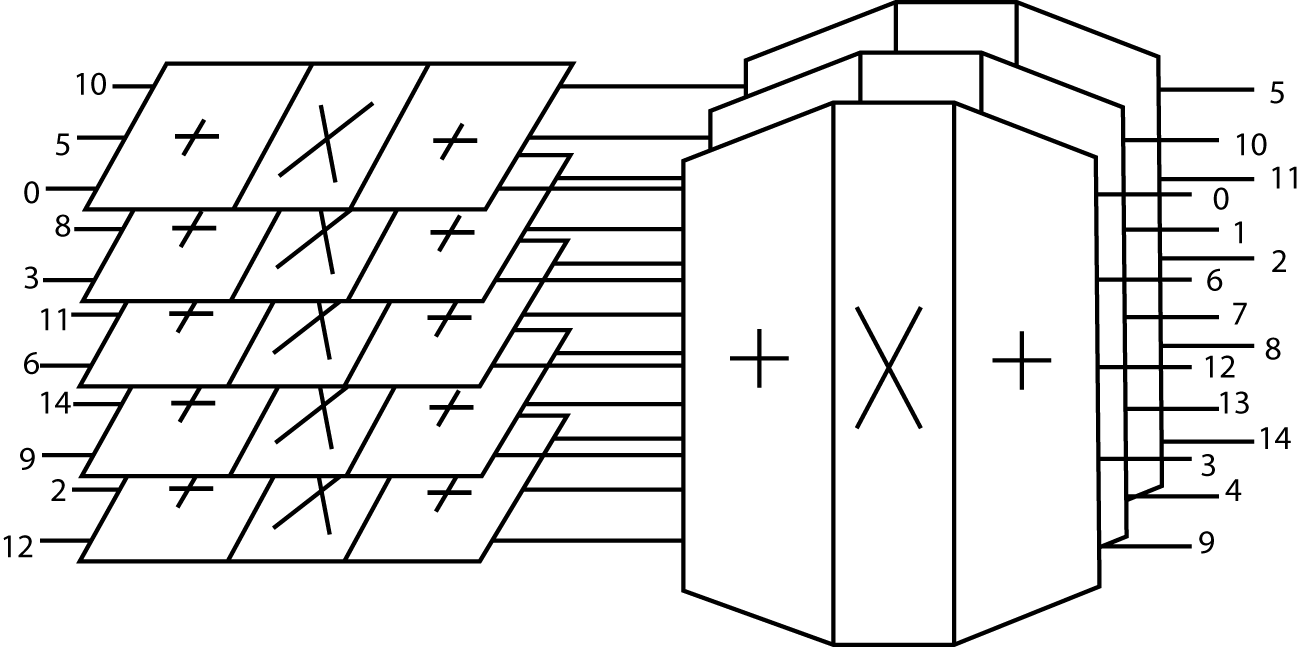
If N is factored into three factors, the DFT of Equation 10.8 would have three nested summations and would be a three-dimensional DFT. This principle extends to any number of factors; however, recall that the Type-1 map requires that all the factors be relatively prime. A very simple three-loop indexing scheme has been developed 1 which gives a compact, efficient PFA program for any number of factors. The basic program structure is illustrated in screen with the short DFT's being omitted for clarity. Complete programs are given in 3 and in the appendices.

C---------------PFA INDEXING LOOPS--------------
                DO 10 K = 1, M
                   N1 = NI(K)
                   N2 = N/N1
                   I(1) = 1
                   DO 20 J = 1, N2
                      DO 30 L=2, N1
                         I(L) = I(L-1) + N2
                         IF (I(L .GT.N)  I(L) = I(L) - N
           30         CONTINUE
                      GOTO (20,102,103,104,105), N1
                      I(1) = I(1) + N1
           20      CONTINUE
           10   CONTINUE
                RETURN
        C----------------MODULE FOR N=2-----------------
          102   R1       = X(I(1))
                X(I(1))  = R1 + X(I(2))
                X(I(2))  = R1 - X(I(2))
                R1       = Y(I(1))
                Y(I(1))  = R1 + Y(I(2))
                Y(I(2))  = R1 - Y(I(2))
                GOTO 20
        C----------------OTHER MODULES------------------
          103   Length-3 DFT
          104   Length-4 DFT
          105   Length-5 DFT
                etc.
 
 

As in the Cooley-Tukey program, the DO 10 loop steps through the M stages (factors of N) and the DO 20 loop calculates the N/N1 length-N1 DFT's. The input index map of Equation 10.6 is implemented in the DO 30 loop and the statement just before label 20. In the PFA, each stage or factor requires a separately programmed module or butterfly. This lengthens the PFA program but an efficient Cooley-Tukey program will also require three or more butterflies.

Because the PFA is calculated in-place using the input index map, the output is scrambled. There are five approaches to dealing with this scrambled output. First, there are some applications where the output does not have to be unscrambled as in the case of high-speed convolution. Second, an unscrambler can be added after the PFA to give the output in correct order just as the bit-reversed-counter is used for the Cooley-Tukey FFT. A simple unscrambler is given in 3, 1 but it is not in place. The third method does the unscrambling in the modules while they are being calculated. This is probably the fastest method but the program must be written for a specific length 3, 1. A fourth method is similar and achieves the unscrambling by choosing the multiplier constants in the modules properly 11. The fifth method uses a separate indexing method for the input and output of each module 3, 17.

The Winograd Fourier transform algorithm (WFTA) uses a very powerful property of the Type-1 index map and the DFT to give a further reduction of the number of multiplications in the PFA. Using an operator notation where F₁ represents taking row DFT's and F₂ represents column DFT's, the two-factor PFA of Equation 10.8 is represented by

(10.9)

It has been shown 21, 9 that if each operator represents identical operations on each row or column, they commute. Since F₁ and F₂ represent length N₁ and N₂ DFT's, they commute and Equation 10.9 can also be written

(10.10)

If each short DFT in F is expressed by three operators as in Winograd’s Short DFT Algorithms: Equation 8 and Winograd’s Short DFT Algorithms: Figure 2, F can be factored as

where A represents the set of additions done on each row or column that performs the residue reduction as Winograd’s Short DFT Algorithms: Equation 30. Because of the appearance of the flow graph of A and because it is the first operator on x, it is called a preweave operator 15. D is the set of M multiplications and A^T (or B^T or C^T) from Winograd’s Short DFT Algorithms: Equation 5 or Winograd’s Short DFT Algorithms: Equation 6 is the reconstruction operator called the postweave. Applying Equation 10.11 to Equation 10.9 gives

(10.12)

This is the PFA of Equation 10.8 and Figure 10.1 where A₁D₁A₁ represents the row DFT's on the array formed from x. Because these operators commute, Equation 10.12 can also be written as

(10.13)

or

(10.14)

but the two adjacent multiplication operators can be premultiplied and the result represented by one operator which is no longer the same for each row or column. Equation Equation 10.14 becomes

(10.15)

This is the basic idea of the Winograd Fourier transform algorithm. The commuting of the multiplication operators together in the center of the algorithm is called nesting and it results in a significant decrease in the number of multiplications that must be done at the execution of the algorithm. Pictorially, the PFA of Figure 10.1 becomes 12 the WFTA in Figure 10.2.

Figure 10.2. 

A Length-15 WFTA with Nested Multiplications

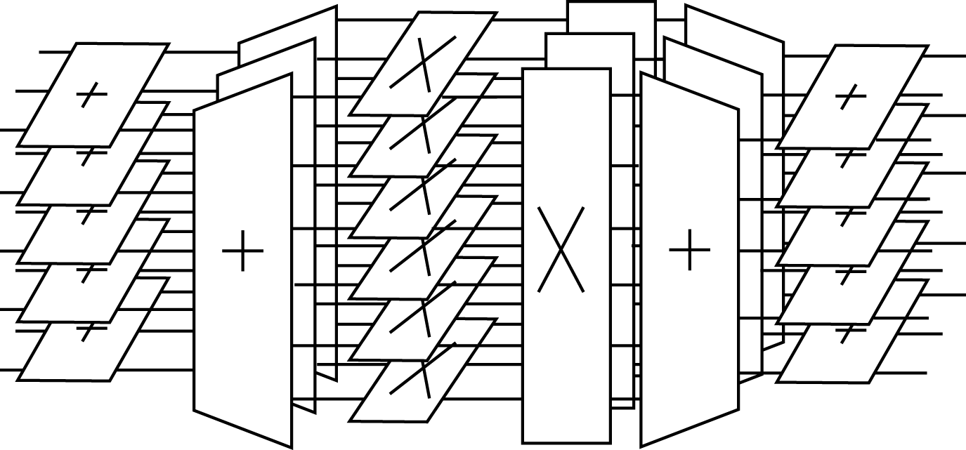
The rectangular structure of the preweave addition operators causes an expansion of the data in the center of the algorithm. The 15 data points in Figure 10.2 become 18 intermediate values. This expansion is a major problem in programming the WFTA because it prevents a straightforward in-place calculation and causes an increase in the number of required additions and in the number of multiplier constants that must be precalculated and stored.

From Figure 10.2 and the idea of premultiplying the individual multiplication operators, it can be seen why the multiplications by unity had to be considered in Winograd’s Short DFT Algorithms: Table 1. Even if a multiplier in D₁ is unity, it may not be in D₂D₁. In Figure 10.2 with factors of three and five, there appear to be 18 multiplications required because of the expansion of the length-5 preweave operator, A₂, however, one of multipliers in each of the length three and five operators is unity, so one of the 18 multipliers in the product is unity. This gives 17 required multiplications - a rather impressive reduction from the 15²=225 multiplications required by direct calculation. This number of 17 complex multiplications will require only 34 real multiplications because, as mentioned earlier, the multiplier constants are purely real or imaginary while the 225 complex multiplications are general and therefore will require four times as many real multiplications.

The number of additions depends on the order of the pre- and postweave operators. For example in the length-15 WFTA in Figure 10.2, if the length-5 had been done first and last, there would have been six row addition preweaves in the preweave operator rather than the five shown. It is difficult to illustrate the algorithm for three or more factors of N, but the ideas apply to any number of factors. Each length has an optimal ordering of the pre- and postweave operators that will minimize the number of additions.

A program for the WFTA is not as simple as for the FFT or PFA because of the very characteristic that reduces the number of multiplications, the nesting. A simple two-factor example program is given in 3 and a general program can be found in 15, 5. The same lengths are possible with the PFA and WFTA and the same short DFT modules can be used, however, the multiplies in the modules must occur in one place for use in the WFTA.

In the previous section it was seen how using the permutation property of the elementary operators in the PFA allowed the nesting of the multiplications to reduce their number. It was also seen that a proper ordering of the operators could minimize the number of additions. These ideas have been extended in formulating a more general algorithm optimizing problem. If the DFT operator F in Equation 10.11 is expressed in a still more factored form obtained from Winograd’s Short DFT Algorithms: Equation 30, a greater variety of ordering can be optimized. For example if the A operators have two factors

(10.16)

The DFT in Equation 10.10 becomes

The operator notation is very helpful in understanding the central ideas, but may hide some important facts. It has been shown 21, 11 that operators in different F_i commute with each other, but the order of the operators within an F_i cannot be changed. They represent the matrix multiplications in Winograd’s Short DFT Algorithms: Equation 30 or Winograd’s Short DFT Algorithms: Equation 8 which do not commute.

This formulation allows a very large set of possible orderings, in fact, the number is so large that some automatic technique must be used to find the “best". It is possible to set up a criterion of optimality that not only includes the number of multiplications but the number of additions as well. The effects of relative multiply-add times, data transfer times, CPU register and memory sizes, and other hardware characteristics can be included in the criterion. Dynamic programming can then be applied to derive an optimal algorithm for a particular application 9. This is a very interesting idea as there is no longer a single algorithm, but a class and an optimizing procedure. The challenge is to generate a broad enough class to result in a solution that is close to a global optimum and to have a practical scheme for finding the solution.

Results obtained applying the dynamic programming method to the design of fairly long DFT algorithms gave algorithms that had fewer multiplications and additions than either a pure PFA or WFTA 9. It seems that some nesting is desirable but not total nesting for four or more factors. There are also some interesting possibilities in mixing the Cooley-Tukey with this formulation. Unfortunately, the twiddle factors are not the same for all rows and columns, therefore, operations cannot commute past a twiddle factor operator. There are ways of breaking the total algorithm into horizontal paths and using different orderings along the different paths 16,