Although there are a wide range of fast Fourier transform (FFT) algorithms, involving a wealth of mathematics from number theory to polynomial algebras, the vast majority of FFT implementations in practice employ some variation on the Cooley-Tukey algorithm 9. The Cooley-Tukey algorithm can be derived in two or three lines of elementary algebra. It can be implemented almost as easily, especially if only power-of-two sizes are desired; numerous popular textbooks list short FFT subroutines for power-of-two sizes, written in the language du jour. The implementation of the Cooley-Tukey algorithm, at least, would therefore seem to be a long-solved problem. In this chapter, however, we will argue that matters are not as straightforward as they might appear.

For many years, the primary route to improving upon the Cooley-Tukey FFT seemed to be reductions in the count of arithmetic operations, which often dominated the execution time prior to the ubiquity of fast floating-point hardware (at least on non-embedded processors). Therefore, great effort was expended towards finding new algorithms with reduced arithmetic counts 13, from Winograd's method to achieve Θ(n) multiplications^[2] (at the cost of many more additions) 54, 22, 12, 13 to the split-radix variant on Cooley-Tukey that long achieved the lowest known total count of additions and multiplications for power-of-two sizes 56, 10, 53, 32, 13 (but was recently improved upon 27, 31). The question of the minimum possible arithmetic count continues to be of fundamental theoretical interest—it is not even known whether better than Θ(nlogn) complexity is possible, since Ω(nlogn) lower bounds on the count of additions have only been proven subject to restrictive assumptions about the algorithms 33, 36, 37. Nevertheless, the difference in the number of arithmetic operations, for power-of-two sizes n, between the 1965 radix-2 Cooley-Tukey algorithm (∼5nlog₂n 9) and the currently lowest-known arithmetic count ( 27, 31) remains only about 25%.

Figure 11.1. 

The ratio of speed (1/time) between a highly optimized FFT (FFTW 3.1.2 15, 16) and a typical textbook radix-2 implementation (Numerical Recipes in C38) on a 3 GHz Intel Core Duo with the Intel C compiler 9.1.043, for single-precision complex-data DFTs of size n, plotted versus log₂n. Top line (squares) shows FFTW with SSE SIMD instructions enabled, which perform multiple arithmetic operations at once (see section ); bottom line (circles) shows FFTW with SSE disabled, which thus requires a similar number of arithmetic instructions to the textbook code. (This is not intended as a criticism of Numerical Recipes—simple radix-2 implementations are reasonable for pedagogy—but it illustrates the radical differences between straightforward and optimized implementations of FFT algorithms, even with similar arithmetic costs.) For n≳2¹⁹, the ratio increases because the textbook code becomes much slower (this happens when the DFT size exceeds the level-2 cache).

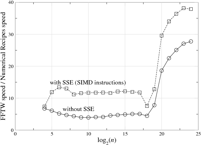
And yet there is a vast gap between this basic mathematical theory and the actual practice—highly optimized FFT packages are often an order of magnitude faster than the textbook subroutines, and the internal structure to achieve this performance is radically different from the typical textbook presentation of the “same” Cooley-Tukey algorithm. For example, Figure 11.1 plots the ratio of benchmark speeds between a highly optimized FFT 15, 16 and a typical textbook radix-2 implementation 38, and the former is faster by a factor of 5–40 (with a larger ratio as n grows). Here, we will consider some of the reasons for this discrepancy, and some techniques that can be used to address the difficulties faced by a practical high-performance FFT implementation.^[3]

In particular, in this chapter we will discuss some of the lessons learned and the strategies adopted in the FFTW library. FFTW 15, 16 is a widely used free-software library that computes the discrete Fourier transform (DFT) and its various special cases. Its performance is competitive even with manufacturer-optimized programs 16, and this performance is portable thanks the structure of the algorithms employed, self-optimization techniques, and highly optimized kernels (FFTW's codelets) generated by a special-purpose compiler.

This chapter is structured as follows. First "Review of the Cooley-Tukey FFT", we briefly review the basic ideas behind the Cooley-Tukey algorithm and define some common terminology, especially focusing on the many degrees of freedom that the abstract algorithm allows to implementations. Next, in "Goals and Background of the FFTW Project", we provide some context for FFTW's development and stress that performance, while it receives the most publicity, is not necessarily the most important consideration in the implementation of a library of this sort. Third, in "FFTs and the Memory Hierarchy", we consider a basic theoretical model of the computer memory hierarchy and its impact on FFT algorithm choices: quite general considerations push implementations towards large radices and explicitly recursive structure. Unfortunately, general considerations are not sufficient in themselves, so we will explain in "Adaptive Composition of FFT Algorithms" how FFTW self-optimizes for particular machines by selecting its algorithm at runtime from a composition of simple algorithmic steps. Furthermore, "Generating Small FFT Kernels" describes the utility and the principles of automatic code generation used to produce the highly optimized building blocks of this composition, FFTW's codelets. Finally, we will briefly consider an important non-performance issue, in "Numerical Accuracy in FFTs".

The (forward, one-dimensional) discrete Fourier transform (DFT) of an array X of n complex numbers is the array Y given by

(11.1)

where 0≤k<n and ω_n=exp(–2πi/n) is a primitive root of unity. Implemented directly, Equation 11.1 would require operations; fast Fourier transforms are O(nlogn) algorithms to compute the same result. The most important FFT (and the one primarily used in FFTW) is known as the “Cooley-Tukey” algorithm, after the two authors who rediscovered and popularized it in 1965 9, although it had been previously known as early as 1805 by Gauss as well as by later re-inventors 24. The basic idea behind this FFT is that a DFT of a composite size n=n₁n₂ can be re-expressed in terms of smaller DFTs of sizes n₁ and n₂—essentially, as a two-dimensional DFT of size n₁×n₂ where the output is transposed. The choices of factorizations of n, combined with the many different ways to implement the data re-orderings of the transpositions, have led to numerous implementation strategies for the Cooley-Tukey FFT, with many variants distinguished by their own names 13, 52. FFTW implements a space of many such variants, as described in "Adaptive Composition of FFT Algorithms", but here we derive the basic algorithm, identify its key features, and outline some important historical variations and their relation to FFTW.

The Cooley-Tukey algorithm can be derived as follows. If n can be factored into n=n₁n₂, Equation 11.1 can be rewritten by letting ℓ=ℓ₁n₂+ℓ₂ and k=k₁+k₂n₁. We then have:

(11.2)

where k_1,2=0,...,n_1,2–1. Thus, the algorithm computes n₂ DFTs of size n₁ (the inner sum), multiplies the result by the so-called 21 twiddle factors , and finally computes n₁ DFTs of size n₂ (the outer sum). This decomposition is then continued recursively. The literature uses the term radix to describe an n₁ or n₂ that is bounded (often constant); the small DFT of the radix is traditionally called a butterfly.

Many well-known variations are distinguished by the radix alone. A decimation in time ( DIT) algorithm uses n₂ as the radix, while a decimation in frequency ( DIF) algorithm uses n₁ as the radix. If multiple radices are used, e.g. for n composite but not a prime power, the algorithm is called mixed radix. A peculiar blending of radix 2 and 4 is called split radix, which was proposed to minimize the count of arithmetic operations 56, 10, 53, 32, 13 although it has been superseded in this regard 27, 31. FFTW implements both DIT and DIF, is mixed-radix with radices that are adapted to the hardware, and often uses much larger radices (e.g. radix 32) than were once common. On the other end of the scale, a “radix” of roughly has been called a four-step FFT algorithm (or six-step, depending on how many transposes one performs) 2; see "FFTs and the Memory Hierarchy" for some theoretical and practical discussion of this algorithm.

A key difficulty in implementing the Cooley-Tukey FFT is that the n₁ dimension corresponds to discontiguous inputs ℓ₁ in X but contiguous outputs k₁ in Y, and vice-versa for n₂. This is a matrix transpose for a single decomposition stage, and the composition of all such transpositions is a (mixed-base) digit-reversal permutation (or bit-reversal, for radix 2). The resulting necessity of discontiguous memory access and data re-ordering hinders efficient use of hierarchical memory architectures (e.g., caches), so that the optimal execution order of an FFT for given hardware is non-obvious, and various approaches have been proposed.

Figure 11.2. 

Schematic of traditional breadth-first (left) vs. recursive depth-first (right) ordering for radix-2 FFT of size 8: the computations for each nested box are completed before doing anything else in the surrounding box. Breadth-first computation performs all butterflies of a given size at once, while depth-first computation completes one subtransform entirely before moving on to the next (as in the algorithm below).

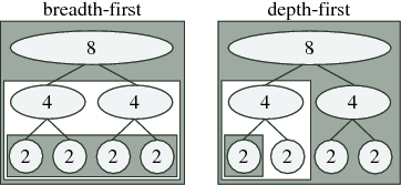
One ordering distinction is between recursion and iteration. As expressed above, the Cooley-Tukey algorithm could be thought of as defining a tree of smaller and smaller DFTs, as depicted in Figure 11.2; for example, a textbook radix-2 algorithm would divide size n into two transforms of size n/2, which are divided into four transforms of size n/4, and so on until a base case is reached (in principle, size 1). This might naturally suggest a recursive implementation in which the tree is traversed “depth-first” as in Figure 11.2(right) and the algorithm of screen—one size n/2 transform is solved completely before processing the other one, and so on. However, most traditional FFT implementations are non-recursive (with rare exceptions 46) and traverse the tree “breadth-first” 52 as in Figure 11.2(left)—in the radix-2 example, they would perform n (trivial) size-1 transforms, then n/2 combinations into size-2 transforms, then n/4 combinations into size-4 transforms, and so on, thus making log₂n passes over the whole array. In contrast, as we discuss in "Discussion", FFTW employs an explicitly recursive strategy that encompasses both depth-first and breadth-first styles, favoring the former since it has some theoretical and practical advantages as discussed in "FFTs and the Memory Hierarchy".

Y[0,...,n–1]←recfft 2(n,X,ι):
IF n=1 THEN
     Y[0]←X[0]
ELSE
     Y[0,...,n/2–1]←recfft2(n/2,X,2ι)
     Y[n/2,...,n–1]←recfft2(n/2,X+ι,2ι)
     FOR k1=0 TO (n/2)–1 DO
          
     END FOR
END IF

A second ordering distinction lies in how the digit-reversal is performed. The classic approach is a single, separate digit-reversal pass following or preceding the arithmetic computations; this approach is so common and so deeply embedded into FFT lore that many practitioners find it difficult to imagine an FFT without an explicit bit-reversal stage. Although this pass requires only O(n) time 29, it can still be non-negligible, especially if the data is out-of-cache; moreover, it neglects the possibility that data reordering during the transform may improve memory locality. Perhaps the oldest alternative is the Stockham auto-sort FFT 47, 52, which transforms back and forth between two arrays with each butterfly, transposing one digit each time, and was popular to improve contiguity of access for vector computers 48. Alternatively, an explicitly recursive style, as in FFTW, performs the digit-reversal implicitly at the “leaves” of its computation when operating out-of-place (see section "Discussion"). A simple example of this style, which computes in-order output using an out-of-place radix-2 FFT without explicit bit-reversal, is shown in the algorithm of screen [corresponding to Figure 11.2(right)]. To operate in-place with O(1) scratch storage, one can interleave small matrix transpositions with the butterflies 26, 49, 40, 23, and a related strategy in FFTW 16 is briefly described by "Discussion".

Finally, we should mention that there are many FFTs entirely distinct from Cooley-Tukey. Three notable such algorithms are the prime-factor algorithm for 35, along with Rader's 41 and Bluestein's 4, 43, 35 algorithms for prime n. FFTW implements the first two in its codelet generator for hard-coded n