• Launch Capacity
• Minimum Spacings between Orbital Vehicles
• Incliment Weather on Earth
• Unfavorable Celestial Conditions


Fundamentals of Transportation/Queueing
91
Examples
Example 1
Problem:
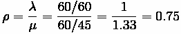
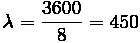
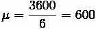
At the Krusty-Burger, if the arrival rate is 1 customer every minute and the
service rate is 1 customer every 45 seconds, find the average queue size, the
average waiting time, and average total delay. Assume an M/M/1 process.
Solution:
To proceed, we convert everything to minutes.
Service time:
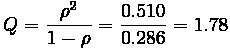
Average queue size (Q):
(within rounding error)
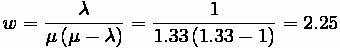
Average wait time:
Average delay time:
Comparison:
We can compute the same results using the M/D/1 equations, the results are shown in the
Table below.
Comparison of M/D/1 and M/M/1 queue properties
''
M/D/1
M/M/1
Q (average queue size (#))
1.125
2.25
w (average waiting time)
1.125
2.25
t (average total delay)
1.88
3
As can be seen, the delay associated with the more random case (M/M/1, which has both
random arrivals and random service) is greater than the less random case (M/D/1), which is to be expected.


Fundamentals of Transportation/Queueing
92
Example 2
Problem:
How likely was it that Homer got his pile of hamburgers in less than 1, 2, or 3
minutes?
Solution:
Example 3
Problem:
Before he encounters the “pimply faced teen” who servers burgers, what is the
likelihood that Homer waited more than 3 minutes?
Solution:
Example 4
Problem:
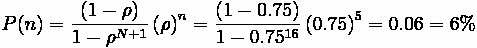
How likely is it that there were more than 5 customers in front of Homer?
Solution:
Fundamentals of Transportation/Queueing
93
Thought Question
Problem
How does one minimize wait time at a queue?
Solution
Cutting in line always helps, but this problem will be answered without breaking any rules.
Think about going out to dinner, only to find a long line at your favorite restaurant. How do you deal with that? Maybe nothing can be done at that time, but the next time you go to
that restaurant, you might pick a new time. Perhaps an earlier one to avoid the lunch or dinner rush. Similar decisions can be seen in traffic. People that are tired of being in network queues on their way to work may attempt to leave earlier or (if possible) later than rush hour to decrease their own travel time. This typically works well until all the other drivers figure out the same thing and shift congestion to a different time.
Sample Problems
Sample Problem 1 : Queueing at a Tollbooth
Sample Problem 2 : Queueing at a Ramp Meter
Sample Problem 3 : Queueing at a Ramp Meter
Variables
• A(t) = λ - Arrival Rate
• D(t) = μ - Departure Rate
• 1/μ - service time
• ρ = λ/ μ - Utilization
• Q - average queue size including customers currently being served (in number of units)
• w - average wait time
• t - average delay time (queue time + service time)
Key Terms
• Queueing theory
• Cumulative input-output diagram (Newell diagram)
• average queue length
• average waiting time
• average total delay time in system
• arrival rate, departure rate
• undersaturated, oversaturated
• D/D/1, M/D/1, M/M/1
• Channels
• Poisson distribution,


Fundamentals of Transportation/Queueing
94
• service rate
• finite (capacitated) queues, infinite (uncapacitated) queues
External Excercises
The assignment seeks to provide students with the opportunity to gain a better
understanding of two queuing theories: M/D/1 and M/M/1. Two preformatted spreadsheets
have been made available for assistance in computing the values sought after in this
excercise. While these spreadsheets provide the computations for these results, the formula is listed below for reference:
Where:
•
: Average customer delay in the queue
•
: Coefficient of variation (CV) of the arrival distribution
•
: Coefficient of variation of the departure distribution
•
: Standard deviation/mean; CV = (1/SqRt (mean)) for Poisson process and CV = 0 for
constant distribution
•
: Average departure rate
•
: Average arrival rate
•
: Utilization = Arrival rate/service rate
M/D/1 Queueing
Download the file for M/D/1 Queueing from the University of Minnesota's STREET website:
M/D/1 Queue Spreadsheet [3]
With this spreadsheet, run 5 simulations for each of the 10 scenarios, using the arrival and departure information listed in the table below. In other words, program the same data into the spreadsheet 5 different times to capture a changing seed and, thus, produce slightly different answers because of the model's sensitivity. A total of 50 simulations will be run.
Scenario
1
2
3
4
5
6
7
8
9
10
Arrival Rate
0.01
0.025
0.05
0.1
0.2
0.3
0.4
0.5
0.6
0.7
Service Rate
0.5
0.5
0.5
0.5
0.5
0.5
0.5
0.5
0.5
0.5
Also, find the utilization for all ten scenarios. Based on the utilization and the distribution variability, use the above equation to compute the average delays for all scenarios with utilization values of less than 1.
Finally, summarize the average-delays obtained both from the simulation and from the WTq equation in the same delay-utilization plot. Interpret your results. How does the average user delay change as utilization increases? Does the above equation provide a satisfactory approximation of the average delays?
M/M/1 Queueing
Download the file for M/M/1 Queueing from the University of Minnesota's STREET website:
M/M/1 Queue Spreadsheet [4]
With this spreadsheet, run 5 simulations for each of the 10 scenarios, using the arrival and departure information listed in the table below. In other words, program the same data into the spreadsheet 5 different times to capture a changing seed and, thus, produce slightly Fundamentals of Transportation/Queueing
95
different answers because of the model's sensitivity. A total of 50 simulations will be run.
Scenario
1
2
3
4
5
6
7
8
9
10
Arrival Rate
0.01
0.025
0.05
0.1
0.2
0.3
0.4
0.5
0.6
0.7
Service Rate
0.5
0.5
0.5
0.5
0.5
0.5
0.5
0.5
0.5
0.5
Again, you need to use five different random seeds for each scenario. Summarize the
results in a delay-utilization plot. Interpret your results (You do NOT need to use the WTq equation given above to compute delays for the M/M/1 queue).
Additional Questions
• Finally compare the M/M/1 queue and the M/D/1 queue. What conclusion can you draw?
(For the same average arrival rate, do users experience the same delays in the two
queuing systems? Why or why not?).
• Provide a brief example where M/M/1 might be the appropriate model to use.
• Provide a brief example where M/D/1 might be the appropriate model to use.
End Notes
Queueing is the only common English word with 5 vowels in a row.
It has been posited: Cooeeing - To call out “cooee,” which is apparently something done in Australia.
The uncommon word: archaeoaeolotropic has 6 vowels - a prehistorical item that is
unequally elastic in different directions - One suspects it is just made up to have a word with 6 vowels in a row though, and the “ae” is questionable anyway.
[2] http://en.wikipedia.org/wiki/Little's_Law
[3] http://street.umn.edu/FOT/MD1Queue.xls
[4] http://street.umn.edu/FOT/MM1Queue.xls


Fundamentals of Transportation/Queueing/Problem1
96
Fundamentals of Transportation/
Queueing/Problem1
Problem:
Application of Single-Channel Undersaturated Infinite Queue Theory to
Tollbooth Operation. Poisson Arrival, Negative Exponential Service Time
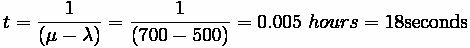
• Arrival Rate = 500 vph,
• Service Rate = 700 vph
Determine
• Percent of Time operator will be free
• Average queue size in system
• Average wait time for vehicles that wait
Note: For operator to be free, vehicles must be 0
• Solution
Fundamentals of Transportation/
Queueing/Solution1
Problem:
Application of Single-Channel Undersaturated Infinite Queue Theory to
Tollbooth Operation. Poisson Arrival, Negative Exponential Service Time
• Arrival Rate = 500 vph,
• Service Rate = 700 vph
Determine
• Percent of Time operator will be free
• Average queue size in system
• Average wait time for vehicles that wait
Note: For operator to be free, vehicles must be 0


Fundamentals of Transportation/Queueing/Solution1
97
Fundamentals of Transportation/
Queueing/Problem2
Problem:
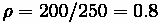
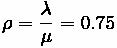
A ramp has an arrival rate of 200 cars an hour and the ramp meter only permits
250 cars per hour, while the ramp can store 40 cars before spilling over.
(A) What is the probability that it is half-full, empty, full?
(B) How many cars do we expect on the ramp?
• Solution
Fundamentals of Transportation/
Queueing/Solution2
Problem:
A ramp has an arrival rate of 200 cars an hour and the ramp meter only permits
250 cars per hour, while the ramp can store 40 cars before spilling over.
(A) What is the probability that it is half-full, empty, full?
(B) How many cars do we expect on the ramp?
Solution:
Part (A)
What is the probability that it is half-full, empty, full?
Half-full
Empty
Full
Part (B)
How many cars do we expect on the ramp?


Fundamentals of Transportation/Queueing/Solution2
98
Fundamentals of Transportation/
Queueing/Problem3
Problem:
In this problem we apply the properties of capacitated queues to an expressway
ramp. Note the following
• Ramp will hold 15 vehicles
• Vehicles can enter expressway at 1 vehicle every 6 seconds
• Vehicles arrive at ramp at 1 vehicle every 8 seconds
Determine:
(A) Probability of 5 cars,
(B) Percent of Time Ramp is Full,
(C) Expected number of vehicles on ramp in peak hour.
• Solution
Fundamentals of Transportation/
Queueing/Solution3
Problem:
In this problem we apply the properties of capacitated queues to an expressway
ramp. Note the following:
• Ramp will hold 15 vehicles
• Vehicles can enter expressway at 1 vehicle every 6 seconds
• Vehicles arrive at ramp at 1 vehicle every 8 seconds
Determine:
(A) Probability of 5 cars,
(B) Percent of Time Ramp is Full,
(C) Expected number of vehicles on ramp in peak hour.
Solution:


Fundamentals of Transportation/Queueing/Solution3
99
Part A
Probability of 5 cars,
Part B
Percent of time ramp is full (i.e. 15 cars),
Part C
Expected number of vehicles on ramp in peak hour.
Conclusion, ramp is large enough to hold most queues, though 12 seconds an hour, there
will be some ramp spillover. It is a policy question as to whether that is acceptable.
Fundamentals of Transportation/
Traffic Flow
Traffic Flow is the study of the movement of individual drivers and vehicles between two points and the interactions they make with one another. Unfortunately, studying traffic flow is difficult because driver behavior is something that cannot be predicted with one-hundred percent certainty. Fortunately, drivers tend to behave within a reasonably consistent range and, thus, traffic streams tend to have some reasonable consistency and can be roughly
represented mathematically. To better represent traffic flow, relationships have been
established between the three main characteristics: (1) flow, (2) density, and (3) velocity.
These relationships help in planning, design, and operations of roadway facilities.


Fundamentals of Transportation/Traffic Flow
100
Traffic flow theory
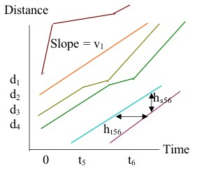
Time-Space Diagram
Traffic engineers represent the
location of a specific vehicle at a
certain time with a time-space
diagram. This two-dimensional
diagram shows the trajectory of a
vehicle through time as it moves
from a specific origin to a specific
destination. Multiple vehicles can
be represented on a diagram and,
thus, certain characteristics, such
as flow at a certain site for a
certain time, can be determined.
Flow and Density
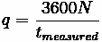
Flow (q) = the rate at which
vehicles pass a fixed point
(vehicles per hour)
Time-space diagram showing trajectories of vehicles over time
and space
Density (Concentration) (k) = number of vehicles (N) over a stretch of roadway (L) (in units of vehicles per kilometer) [1]
where:
•
= number of vehicles passing a point in the roadway in
sec
•
= equivalent hourly flow
•
= length of roadway
•
= density
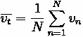
Speed
Measuring speed of traffic