


Fundamentals of Transportation/Shockwaves
116
Relative speed
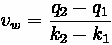
With
equal to the space mean speed of vehicles in area 1, the speed relative to the line
is:
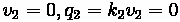
The speed of vehicles in area 2 relative to the line w is
Boundary crossing
The number of vehicles crossing line 2 from area 1 during time period is
and similarly
By conservation of flow, the number of vehicles crossing from left equals the number that crossed on the right
so:
or
which is equivalent to
Examples
Example 1
• (A) What is the wave speed (
)?
• (B) What is the rate at which the queue grows, in units of vehicles per hour ( )?
Solution:
(A) At what rate does the queue increase?
1. Identify Unknowns:
2. Solve for wave speed (
)
Conclusion: the queue grows against traffic
(B) What is the rate at which the queue grows, in units of vehicles per hour?


Fundamentals of Transportation/Shockwaves
117
Thought Question
Problem
Shockwaves are generally something that transportation agencies would like to minimize
on their respective corridor. Shockwaves are considered a safety concern, as the transition of conditions can often lead to accidents, sometimes serious ones. Generally, these
transition zones are problems because of the inherent fallibility of human beings. That is, people are not always giving full attention to the road around them, as they get distracted by a colorful billboard, screaming kids in the backseat, or a flashy sports car in the adjacent lanes. If people were able to give full attention to the road, would these shockwaves still be causing accidents?
Solution
Yes, but not to the same extent. While accidents caused by driver inattentiveness would
decrease nearly to zero, accidents would still be occurring between different vehicle types.
For example, in a case where conditions change very dramatically, a small car (say, a
Beetle) would be able to stop very quickly. A semi truck, however, is a much heavier vehicle and would require a longer distance to stop. If both were moving at the same speed when
encountering the shockwave, the truck may not be able to stop in time before smashing into the vehicle ahead of them. That is why most trucks are seen creeping along through traffic with very big gaps ahead of them.
Sample Problem
Variables
•
- flow
•
- capacity (maximum flow)
•
- density
•
- speed
•
- relative speed (travel speed minus wave speed)
•
- wave speed
•
- number of vehicles crossing wave boundary


Fundamentals of Transportation/Shockwaves
118
Key Terms
• Shockwaves
• Time lag, space lag
References
[1] http://www.vwi.tu-dresden.de/~treiber/movie3d/index.html
[2] http://www.youtube.com/watch?v=Suugn-p5C1M
Fundamentals of Transportation/
Shockwaves/Problem
Problem:
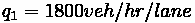
Flow on a road is
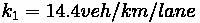
, and the density of
. To
reduce speeding on a section of highway, a police cruiser decides to implement a rolling roadblock, and to travel in the left lane at the speed limit (
) for 10 km. No
one dares pass. After the police cruiser joins, the platoon density increases to 20
veh/km/lane and flow drops. How many vehicles (per lane) will be in the platoon when the police car leaves the highway?
• Solution


Fundamentals of Transportation/Shockwaves/Solution
119
Fundamentals of Transportation/
Shockwaves/Solution
Problem:
Flow on a road is
, and the density of
. To
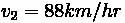
reduce speeding on a section of highway, a police cruiser decides to implement a rolling roadblock, and to travel in the left lane at the speed limit (
) for 10 km. No
one dares pass. After the police cruiser joins, the platoon density increases to 20
veh/km/lane and flow drops. How many vehicles (per lane) will be in the platoon when the police car leaves the highway?
Solution:
Step 0
Solve for Unknowns:
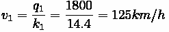
Original speed
Flow after police cruiser joins
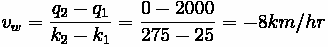
Step 1
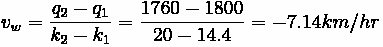
Calculate the wave velocity:
Step 2
Determine the growth rate of the platoon (relative speed)
Step 3
Determine the time spent by the police cruiser on the highway
Step 4
Calculate the Length of platoon (not a standing queue)
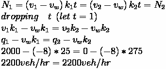
Step 5
What is the rate at which the queue grows, in units of vehicles per hour?
Step 6
The number of vehicles in platoon


Fundamentals of Transportation/Shockwaves/Solution
120
OR
Fundamentals of Transportation/
Traffic Signals
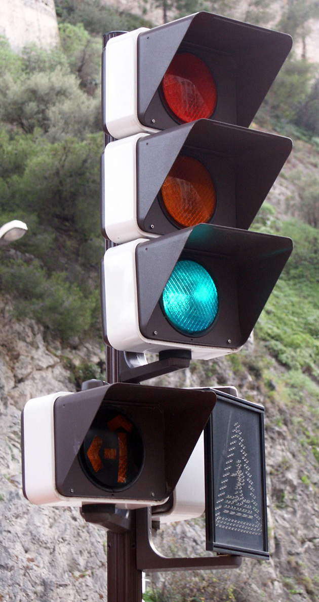
Traffic Signals are one of the more familiar types of
intersection control. Using either a fixed or adaptive
schedule, traffic signals allow certain parts of the
intersection to move while forcing other parts to
wait, delivering instructions to drivers through a set
of colorful lights (generally, of the standard
red-yellow-green format). Some purposes of traffic
signals are to (1) improve overall safety, (2) decrease
average travel time through an intersection, and (3)
equalize the quality of services for all or most traffic
streams. Traffic signals provide orderly movement of
intersection traffic, have the abilities to be flexible
for changes in traffic flow, and can assign priority
treatment to certain movements or vehicles, such as
emergency services. However, they may increase
delay during the off-peak period and increase the
probability of certain accidents, such as rear-end
collisions. Additionally, when improperly configured,
driver irritation can become an issue. Fortunately,
traffic signals are generally a well-accepted form of
traffic control for busy intersections and continue to
be deployed.
A Traffic Light
Intersection Queueing
At an intersection where certain approaches are denied movement, queueing will inherently occur. Of the various queueing models, one of the more commons and simple ones is the
D/D/1 Queueing Model. This model assumes that arrivals and departures are deterministic
and one departure channel exists. D/D/1 is quite intutive and easily solvable. Using this form of queueing with an arrival rate
and a departure rate
, certain useful values
regarding the consequences of queues can be computed.
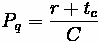
One important piece of information is the duration of the queue for a given approach. This time value can be calculated through the following formula:
Where:
•
= Time for queue to clear
•
= Arrival Rate divided by Departure Rate


Fundamentals of Transportation/Traffic Signals
121
•
= Red Time
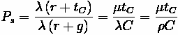
With this, various proportions dealing with queues can be calculated. The first determines the proportion of cycle with a queue.
Where:
•
= Proportion of cycle with a queue
•
= Cycle Lengh
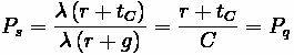
Similarly, the proportion of stopped vehicles can be calculated.
Where:
•
= Proportion of Stopped Vehicles
•
= Green Time
Therefore, the maximum number of vehicles in a queue can be found.
Intersection delay
Various models of intersection delay at isolated intersections have been put forward,
combining queuing theory with empirical observations of various arrival rates and
discharge times (Webster and Cobbe 1966; Hurdle 1985; Hagen and Courage 1992).
Intersections on arterials are more complex phenomena, including factors such as signal
progression and spillover of queues between adjacent intersections. Delay is broken into two parts: uniform delay, which is the delay that would occur if the arrival pattern were uniform, and overflow delay, caused by stochastic variations in the arrival patterns, which manifests itself when the arrival rate exceeds the service flow of the intersection for a time period.
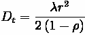
Delay can be computed with knowledge of arrival rates, departure rates, and red times.
Graphically, total delay is the product of all queues over the time period in which they are present.
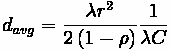
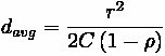
Similarly, average vehicle delay per cycle can be computed.
From this, maximum delay for any vehicle can be found.


Fundamentals of Transportation/Traffic Signals
122
Level of Service
In order to assess the performance of a signalized intersection, a qualitative assessment called Level of Service (LOS) is assessed, based upon quantitative performance measures.
For LOS, the performance measured used is average control delay per vehicle. The general procedure for determining LOS is to calculate lane group capacities, calculate delay, and then make a determination.
Lane group capacities can be calculated through the following equation:
Where:
•
= Lane Group Capacity
•
= Adjusted Saturation Flow Rate
•
= Effective Green Length
•
= Cycle Length
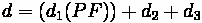
Average control delay per vehicle, thus, can be calculated by summing the types of delay mentioned earlier.
Where:
•
= Average Signal Delay per vehicle (sec)
•
= Average Delay per vehicle due to uniform arrivals (sec)
•
= Progression Adjustment Factor
•
= Average Delay per vehicle due to random arrivals (sec)
•
= Average delay per vehicle due to initial queue at start of analysis time period (sec)
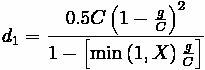
Uniform delay can be calculated through the following formula:
Where:
•
= Volume/Capacity (v/c) ratio for lane group.
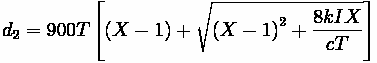
Similarly, random delay can be calculated:
Where:
•
= Duration of Analysis Period (in hours)
•
= Delay Adjustment Factor that is dependent on signal controller mode
•
= Upstream filtering/metering adjustment factor
Overflow delay generally only applies to densely urban corridors, where queues can
sometimes spill over into previous intersections. Since this is not very common (usually the consequence of a poorly timed intersection sequence, the rare increase of traffic demand, or an emergency vehicle passing through the area), it is generally not taken into account for simple problems.
Delay can be calcaulated for individual vehicles in certain approaches or lane groups.
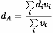
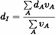
Average delay per vehicle for an approach A can be calculated using the following formula:


Fundamentals of Transportation/Traffic Signals
123
Where:
•
= Average Delay per vehicle for approach A (sec)
•
= Average Delay per vehicle for lane group i on approach A (sec)
•
= Analysis flow rate for lane group i
Average delay per vehicle for the intersection can then be calculated:
Where:
•
= Average Delay per vehicle for the intersection (sec)
•
= Average Delay per vehicle for approach A (sec)
•
= Analysis flow rate for approach A
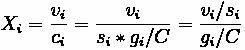
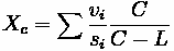
Critical Lane Groups
For any combination of lane group movements, one lane group will dictate the necessary
green time during a particular phase. This lane group is called the Critical Lane Group. This lane group has the highest traffic intensity (v/s) and the allocation of green time for each phase is based on this ratio.
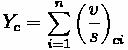
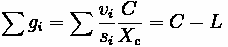
The sum of the flow ratios for the critical lane groups can be used to calculate a suitable cycle length.
Where:
•
= Sum of Flow Ratios for Critical Lane Groups
•
= Flow Ratio for Critical Lane Group i
•
= Number of Critical Lane Groups
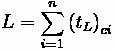
Similarly, the total lost time for the cycle is also an element that can be used in the
calculation of cycle length.
Where:
•
= Total lost Time for Cycle
•
= Total Lost Time for Critical Lane Group i


Fundamentals of Transportation/Traffic Signals
124
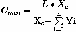
Cycle Length Calcuation
Cycle lengths are calculated by summing individual phase lengths. Using the previous
formulas for assistance, the minimum cycle length necessary for the lane group volumes
and phasing plan can be easily calculated.
Where:
•
= Minimum necessary cycle length
•
= Critical v/c ratio for the intersection
•
= Flow Ratio for Critical Lane Group
•
= Number of Critical Lane Groups
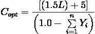
This equation calculates the minimum cycle length necesary for the intersection to operate at an acceptable level, but it does not necessarily minimize the average vehicle delay. A more optimal cycle length usually exists that would minimize average delay. Webster
(1958) proposed an equation for the calculation of cycle length that seeks to minize vehicle delay. This optimum cycle length formula is listed below.
Where:
•
= Optimal Cycle Length for Minimizing Delay
Green Time Allocation
Once cycle length has been determined, the next step is to determine the allocation of
green time to each phase. Several strategi