⎪
B =
,
D =
⎢ ⎥
⎢ K p⎜1+
+
⎟⎥ ,
⎪
⎣ ⎦
1
⎣
⎝
Ti
h ⎠⎦
⎭
Since the predictable description of the system (11)-(12) is not useful for the PID control
algorithm, the system defined by state equation (4), measurement equation (8), modulation
equation (7) and performance index (9) is described at sampling instants in alternative form
x +
(27)
1 =
+ 0 − +1 + 1 − +
k
Fxk
Γ uk l
Γ uk l
k
w
z = ' +
(28)
k
d xk
k
n
where
θ
h θ
−
A( h θ
− )
Γ
(29)
1 = e
eAvbdv = F( h −θ ) g(θ )
,
Γ 0 = eAvbdv = g( h − θ )
∫
∫
0
0
The corresponding state-space description is as follows
⎡ x 1 ⎤ ⎡ F Γ Γ L 0
1
0
⎤ ⎡ x ⎤
⎡0⎤
⎡ I ⎤
k +
k
⎢
⎥ ⎢
⎥ ⎢
⎥
⎢ ⎥
⎢ ⎥
u
0
0
1 L 0
u
⎢
0
0
k − l+1 ⎥
⎢
⎥ ⎢ k− l ⎥
⎢ ⎥
⎢ ⎥ (30)
⎢ M ⎥ = ⎢ M M M O M⎥ ⎢ M ⎥ + ⎢M⎥ u + ⎢M⎥ w
k
k
⎢
⎥ ⎢
⎥ ⎢
⎥
⎢ ⎥
⎢ ⎥
u
0
0
0 L 1
u
⎢
0
0
k −1 ⎥
⎢
⎥ ⎢ k−2 ⎥
⎢ ⎥
⎢ ⎥
⎢ u ⎥ ⎢0 0 0 L 0⎥ ⎢ u ⎥
⎢1⎥
⎢0⎥
⎣ k ⎦ ⎣
⎦ ⎣ k−1 ⎦
1
4
4
4
2
4
4
4
3
3
2
1
{
⎣ ⎦
⎦
{
⎣
F
x
Γ
Ω
k
Introduce the notation
⎡ P
P ⎤ ⎫
P = {
E x , x '} =
k
k
⎢ 11
12 ⎥ ⎪
⎣ P
P
21
22 ⎦
⎪⎪
⎡ x
(31)
k ⎤
⎢
⎥
⎪⎪
uk− l
⎬
⎢
⎥
⎡ xk ⎤
⎪
x =
' x = ⎢ M ⎥
k
⎢ c ⎥
k
⎪
⎣ x k ⎦
⎢
⎥
u
⎪
⎢ k−2 ⎥
⎪
⎢⎣ u ⎥
k −1 ⎦
⎪⎭
Employing (31) and (25), the performance index (13) can be rewritten as
98
New Approaches in Automation and Robotics
I = tr{ Q
τ
1 Fp P 11 Fp +
' Q W
1
( ) } − tr{
c
Fp ' q 12 D d' P 11 }
⎫
− tr{
c
dD ' q 12 ' Fp P 11 }+ tr{
c
c
q 2 dD ' D d' P 11 } ⎪⎪
(32)
+ tr{ c
C ' q 12 ' Fp P 12 }− tr{
c
c
q 2 C ' D d' P 12 }
⎪⎬
+ tr{
c
Fpq 12 C P 21 }− tr{
c
c
q 2 dD C P 21 }
⎪⎪
+ tr{
c
c
q
ν
2 C ' C P 22 } + tr{
c
c
q D ' D 2
2
+ qw}
⎪⎭
4.3 Output and control variances
The output and control variances at sampling instants for the LQG controller can be
calculated from the following expressions
2
σ
= d' E{ x , x ' d
}
= d' X
)
11
(
d
(33)
y LQG
k
k
k
2
c
c
c
c
σ
=
'
{ ˆ , ˆ
=
(34)
u
'}
'
'
(22)
'
k LQG
k FpE x
x
F k
k F X
F k
k k
k k
p
p
p
where
⎡ X
)
11
(
X
)
12
(
⎤ ⎫
X =
{
E x , x '} =
k
k
⎢
⎥ ⎪
⎣ X ( )
21
X ( )
22 ⎦ ⎪⎪
⎡ x
x
k ⎤
⎡ ˆ ⎤
(35)
⎢
⎥
⎢ k k ⎥ ⎪⎪
u
u
k − l
k − l
⎬
⎢
⎡ xk ⎤
⎥
⎢
⎥ ⎪
x =
x
M
x
k
⎢
⎥,
= ⎢
⎥, ˆ = ⎢ M ⎥
ˆ
k
k
x
⎪
k k
⎢
⎣
⎦
⎥
⎢
⎥
u
u
⎪
⎢ k−2⎥
⎢ k−2⎥ ⎪
⎢ u ⎥
⎢
⎣
u
k −1 ⎦
⎣
⎥
k −1 ⎦
⎪⎭
and formulas in case of PID type controllers are defined as follows
2
σ
=
=
(36)
y
var
'
k PID
{ yk} d P 11 d
2
σ u PID =
{
var u
k }
c
c
c
c
= C
k
22
P C −
' D d' 12
P C '
⎪⎫⎬ (37)
− c
c
c
c
c
c
C
ν
21
P dD ' + D d' P dD +
'
2
11
D
D ' ⎪⎭
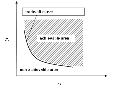
5. Trade-off curves
Relationships in two-dimensional space of such criterions as output and control signal
variances determine the trade-off curve (Huang & Shah 1999) which separate two regions:
achievable (above) and non-achievable (below). On the basis of point location with respect
to the trade-off curve one can assess the control performance. Thus the trade-off curve can
be defined by means the benchmark which minimizes quadratic performance index in the
form of (9). This means that such benchmark acts the lower bound taking the control effort
into account.
Since standard deviations better characterize signal magnitudes, in the chapter trade-off
curves are drawn on the plane std(y)-std(u).
Developments in the Control Loops Benchmarking
99
Therefore the LQG control benchmark for a linear continuous-time plant whose output is
corrupted by a stochastic disturbance controlled by a discrete-time controller is proposed.
The quality of control systems with PID controllers tuned both classically (QDR-Quarter
Decay Ratio) and optimally in such way that disturbance characteristics are taken into
account is investigated and, assuming the same control effort, compared with the
benchmark. It has been shown that optimal tuning of classical PID controllers improves the
disturbance attenuation bringing it closer to the lower bound.
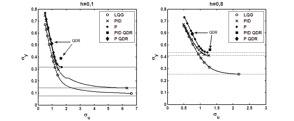
Fig. 1. Trade-off curve
In Fig. 1 standard deviation of output signal against standard deviation of control signal for
systems with LQG and optimally tuned PID type controllers is plotted1. Optimal values of
these parameters were received for varying values of the weighting factor λ.
Results of the minimum variance strategy are plotted as horizontal lines. And results of PID
type control with controllers settings supplied by means of QDR method are plotted as
points.
Fig. 2. Standard deviation of output vs control signal (trade-off curve)
1
p
1
Exemplary plant transfer function:
G ( s) = (α s + ) 1( s + ) ,
1 2
100
New Approaches in Automation and Robotics
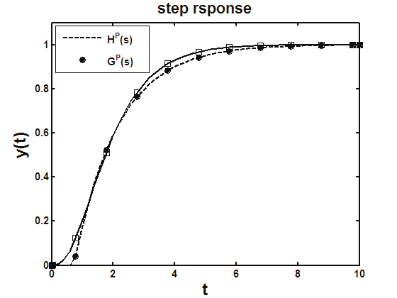
6. Control performance assessment based on lag-delay model
Suitability of control quality assessment based on delay approximation for delay-free plants
is investigated in this section. To this end, the LQG control benchmark, which can be seen as
a MV benchmark with bounded control variance, is compared for both linear delay-free
continuous-time plants with outputs corrupted by a stochastic disturbance and their lag-
delay models. Using approximated plant models, the area of achievable accuracy is then
defined for control performance assessment.
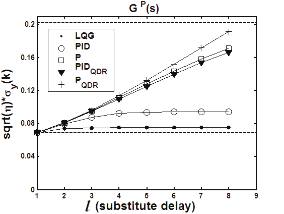
The transfer function GP(s)2 is then approximated by the lag-delay transfer function (3) HP(s).
Comparison of their step responses is given in Fig. 3.
Fig. 3. Step response characteristics of original delay-free plant and its lag-delay model.
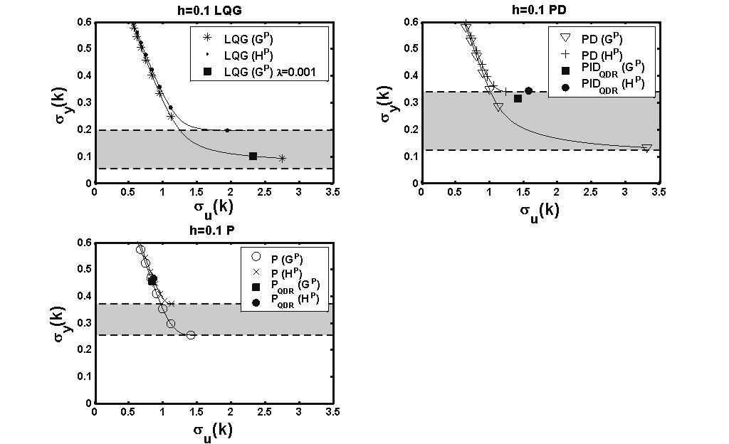
In Fig. 4 standard deviations of output signal against standard deviations of control signal
for both delayed and non-delayed systems controlled by, respectively, optimal LQG and
PID type controllers are plotted. The plots are parametrized by the weighting factor λ.
Results of the MV (λ=0) strategy are plotted as horizontal dashed lines and define areas of
uncertainty of the performance lower bound when using the lag-delay approximation of
non-delayed systems. Results of the benchmark designed for original model with realistic
control signal magnitudes (λ=0.001) and PID type control with controllers settings supplied
by means of QDR methods are plotted as points.
The MV control strategy used for the delayed model gives lower control quality than the
MV algorithm for the delay-free model. Furthermore there is no significant improvement of
control quality when optimal settings for classical controllers are used for the delayed model
as compared to those obtained by means of QDR method.
Since control signal magnitudes of the lower bound i.e. LQG (λ=0) for lag-delay
approximation (3) and those achieved with PID controller are comparable, the most
popular MV benchmark η of (1) makes sense when using delayed models, indicating that
relatively good performance. It can unfortunately hide the possibility of further
performance improvement when delay-free model is used.
2
p
G ( )
1
s = ( s+ ) 1( 5.
0 s + ) 2
1
Developments in the Control Loops Benchmarking
101
Fig. 4. Areas of achievable accuracy using lag-delay approximation.
Table 1 presents the values of index η and standard deviation of output signal σy for the
systems with the plant transfer function GP(s) and HP(s). Furthermore the value of sqrt(η)*σy
is shown which is equivalent to standard deviation of the output signal obtained when pure
MV Astrom’s algorithm is used.
λ=0 h=0.1
η
σy sqrt(η) sqrt(η)*σy
LQG [GP(s)] 0.8421 0.0751 0.9176 0.0689
PD [GP(s)] 0.2668 0.1333 0.5166 0.0689
P [GP(s)] 0.0701 0.2601 0.2648 0.0689
PIDQDR [GP(s)] 0.0480 0.3145 0.2088 0.0689
PQDR [GP(s)] 0.0230 0.4545 0.1517 0.0689
LQG [HP(s)] 0.9998 0.2026 0.9999 0.2026
PD [HP(s)] 0.3465 0.3442 0.5886 0.2026
P [HP(s)] 0.2938 0.3738 0.7362 0.2026
PIDQDR [HP(s)] 0.3485 0.3432 0.5652 0.2026
PQDR [HP(s)] 0.1900 0.4649 0.4359 0.2026
substitute delay
LQG [GP(s)] 1.0000 0.0751 1.0000 0.0751
PD [GP(s)] 0.4992 0.1333 0.7065 0.0942
P [GP(s)] 0.4315 0.2601 0.6568 0.1709
PIDQDR [GP(s)] 0.2799 0.3145 0.5094 0.1664
PQDR [GP(s)] 0.1773 0.4545 0.2791 0.1914
Table 1. Values of performance measure η and estimated output standard deviation under
pure MV Astrom’s control algorithm
102
New Approaches in Automation and Robotics
The bottom part of the table shows the values calculated for the delay-free system, GP(s),
and calculated using the estimated substitute delay. The most important conclusion is that
the use of the substitute delay to assess the system control performance often gives
unreliable results. Another interesting observation is that the values from the last column
belong to the uncertainty area of performance lower bound (see Fig. 3). This can also be
seen from Fig. 5s where the estimates of the performance lower bound are plotted when
assuming different values of delay l.
Fig. 5. Areas of achievable accuracy using lag-delay approximation.
7. More complete characteristic of control error
As mentioned in the previous section using more sophisticated original delay-free model
additional improvement of control quality can be attained for both PID and LQG
controllers. The price paid is much larger control variance. It is interesting to note that while
LQG systems remain robust this is not longer valid for PID controllers.
Then in this section comparison of certain time and frequency domain functions will be
done to give further insight into assessment of control performance in terms of system
robustness.
The notion of 1D-PID will be also used to denote the limited authority tuning of PID
controller whose dynamical parameters Ti and Td are chosen from a popular tuning rule, e.g.
the QDR method based on model (3), remain constant, and only the gain Kp is chosen so as
to minimize the index in (9).
In Fig. 6. trade-off curves displaying standard deviations of output signals against standard
deviations of control signals for the original delay-free system controlled by optimal LQG
controller and by optimally tuned 1D-PID controller are plotted. Plots are parameterized by
the weighting factor λ, and results of the unrestricted MV-LQG and restricted structure, 1D-
PID MV strategies (λ=0) are plotted as horizontal doted lines for both types of controllers.
Due to excessive control actions and small increase of control quality MV based benchmarks
Developments in the Control Loops Benchmarking
103
are not particularly authoritative [3] for non-delayed systems. Therefore, a benchmark
which assumes restricted control effort seems to be more suitable for systems controlled by
the PID controllers. Points a→a1, b→b1, c→c1 depict correspondence of control systems
with the same control effort.
η
√η
a 0.4846 0,6961
b 0.3075 0,5545
c 0.3018 0,5494
a1 0.7932 0,8906
b1 0.7071 0,8409
c1 0.5853 0,7650
Table 2. Performance measure for systems in Fig. 6
It is worth noting that for the MV-LQG η=0.9321 (sqrt(η)=0,9655). The almost MV-LQG
system represented as a1 has the value of η=0.7932 (sqrt(η)=0,8906), and for a reasonably
tuned system represented by c1 there is η=0.5853 (sqrt(η)=0,7650), respectively.
Fig. 6. Standard deviation of output vs control signal for PID and LQG controlled systems.
In Fig. 7-8 PSD3 functions of output signals of corresponding systems are plotted and
compared with the PSDF of disturbance. Important observation is that the optimal PID
controller distinguishes itself by very poor robustness both in terms of phase margin and
large sensitivity peak. This fact is reflected by the appearance o